一、决策树
- 决策树-分类树
  - 重要参数criterion
  - 剪枝参数
    - 7. 调整参数
    - 8. 绘制学习曲线，确定最优参数
- 决策树-回归树
  - 1. 交叉验证cross_val_score的用法
  - 2. 一维回归图像的绘制
二、泰坦尼克号生存预测
- 1. 导入数据集 & 数据预处理
  - 探索数据
2. 提取标签和特征矩阵，分测试集和训练集
3. 导入模型
4. 在不同max_depth下观察模型的拟合情况
5. 用网格搜索调整参数

一、决策树

决策树训练目标是创建一个模型来预测样本的目标值。每个内部节点对应于一个输入属性，子节点代表父节点的属性的可能取值。每个叶子节点代表输入属性得到的可能输出值。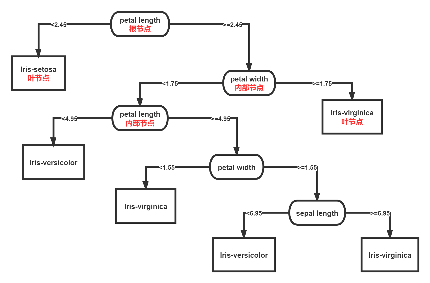
Iris-决策树.png
一棵树的训练过程：根据一个指标，分裂训练集为几个子集。这个过程不断的在产生的子集里重复递归进行，即递归分割。当一个训练子集的类标都相同时递归停止。
数据以如下方式表示:
决策树与泰坦尼克号生存预测 - 图2
其中Y是目标值，向量x由这些属性构成, x, x, x 等等，用来得到目标值。

在决策分析中，一棵决策树可以明确地表达决策的过程。在数据挖掘中， 一棵决策树表达的是数据而不是决策。

与其他的数据挖掘算法相比，决策树有许多 优点 ：

易于理解和解释 人们很容易理解决策树的意义；
只需很少的数据准备 其他技术往往需要数据归一化；
即可以处理数值型数据也可以处理类别型数据 其他技术往往只能处理一种数据类型。例如关联规则只能处理类别型的而神经网络只能处理数值型的数据；
使用白箱模型 输出结果容易通过模型的结构来解释。而神经网络是黑箱模型，很难解释输出的结果；
可以通过测试集来验证模型的性能 可以考虑模型的稳定性；
強健控制 对噪声处理有好的強健性；
可以很好的处理大规模数据

缺点 ：

容易发生过拟合（随机森林可以很大程度上减少过拟合）；
容易忽略数据集中属性的相互关联；
对于那些各类别样本数量不一致的数据，在决策树中，进行属性划分时，不同的判定准则会带来不同的属性选择倾向；信息增益准则对可取数目较多的属性有所偏好（典型代表ID3算法），而增益率准则（CART）则对可取数目较少的属性有所偏好，但CART进行属性划分时候不再简单地直接利用增益率尽心划分，而是采用一种启发式规则）（只要是使用了信息增益，都有这个缺点，如RF）。
ID3算法计算信息增益时结果偏向数值比较多的特征。

决策树-分类树

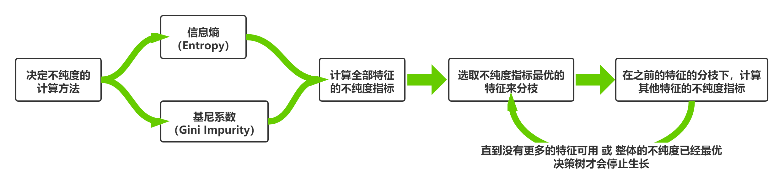
重要参数criterion

决策树参数：criterion.png

1. 导入需要的算法库和模块

from sklearn import tree
from sklearn.datasets import load_wine
from sklearn.model_selection import train_test_split
import pandas as pd

import graphviz

2. 探索数据

wine = load_wine() # 数据实例化
wine # data, target, target_name, DESCR, feature_names

{'data': array([[1.423e+01, 1.710e+00, 2.430e+00, ..., 1.040e+00, 3.920e+00,
         1.065e+03],
        [1.320e+01, 1.780e+00, 2.140e+00, ..., 1.050e+00, 3.400e+00,
         1.050e+03],
        [1.316e+01, 2.360e+00, 2.670e+00, ..., 1.030e+00, 3.170e+00,
         1.185e+03],
        ...,
        [1.327e+01, 4.280e+00, 2.260e+00, ..., 5.900e-01, 1.560e+00,
         8.350e+02],
        [1.317e+01, 2.590e+00, 2.370e+00, ..., 6.000e-01, 1.620e+00,
         8.400e+02],
        [1.413e+01, 4.100e+00, 2.740e+00, ..., 6.100e-01, 1.600e+00,
         5.600e+02]]),
 'target': array([0, 0, 0, 0, 0, 0, 0, 0, 0, 0, 0, 0, 0, 0, 0, 0, 0, 0, 0, 0, 0, 0,
        0, 0, 0, 0, 0, 0, 0, 0, 0, 0, 0, 0, 0, 0, 0, 0, 0, 0, 0, 0, 0, 0,
        0, 0, 0, 0, 0, 0, 0, 0, 0, 0, 0, 0, 0, 0, 0, 1, 1, 1, 1, 1, 1, 1,
        1, 1, 1, 1, 1, 1, 1, 1, 1, 1, 1, 1, 1, 1, 1, 1, 1, 1, 1, 1, 1, 1,
        1, 1, 1, 1, 1, 1, 1, 1, 1, 1, 1, 1, 1, 1, 1, 1, 1, 1, 1, 1, 1, 1,
        1, 1, 1, 1, 1, 1, 1, 1, 1, 1, 1, 1, 1, 1, 1, 1, 1, 1, 1, 1, 2, 2,
        2, 2, 2, 2, 2, 2, 2, 2, 2, 2, 2, 2, 2, 2, 2, 2, 2, 2, 2, 2, 2, 2,
        2, 2, 2, 2, 2, 2, 2, 2, 2, 2, 2, 2, 2, 2, 2, 2, 2, 2, 2, 2, 2, 2,
        2, 2]),
 'target_names': array(['class_0', 'class_1', 'class_2'], dtype='<U7'),
 'DESCR': '.. _wine_dataset:\n\nWine recognition dataset\n------------------------\n\n**Data Set Characteristics:**\n\n    :Number of Instances: 178 (50 in each of three classes)\n    :Number of Attributes: 13 numeric, predictive attributes and the class\n    :Attribute Information:\n \t\t- Alcohol\n \t\t- Malic acid\n \t\t- Ash\n\t\t- Alcalinity of ash  \n \t\t- Magnesium\n\t\t- Total phenols\n \t\t- Flavanoids\n \t\t- Nonflavanoid phenols\n \t\t- Proanthocyanins\n\t\t- Color intensity\n \t\t- Hue\n \t\t- OD280/OD315 of diluted wines\n \t\t- Proline\n\n    - class:\n            - class_0\n            - class_1\n            - class_2\n\t\t\n    :Summary Statistics:\n    \n    ============================= ==== ===== ======= =====\n                                   Min   Max   Mean     SD\n    ============================= ==== ===== ======= =====\n    Alcohol:                      11.0  14.8    13.0   0.8\n    Malic Acid:                   0.74  5.80    2.34  1.12\n    Ash:                          1.36  3.23    2.36  0.27\n    Alcalinity of Ash:            10.6  30.0    19.5   3.3\n    Magnesium:                    70.0 162.0    99.7  14.3\n    Total Phenols:                0.98  3.88    2.29  0.63\n    Flavanoids:                   0.34  5.08    2.03  1.00\n    Nonflavanoid Phenols:         0.13  0.66    0.36  0.12\n    Proanthocyanins:              0.41  3.58    1.59  0.57\n    Colour Intensity:              1.3  13.0     5.1   2.3\n    Hue:                          0.48  1.71    0.96  0.23\n    OD280/OD315 of diluted wines: 1.27  4.00    2.61  0.71\n    Proline:                       278  1680     746   315\n    ============================= ==== ===== ======= =====\n\n    :Missing Attribute Values: None\n    :Class Distribution: class_0 (59), class_1 (71), class_2 (48)\n    :Creator: R.A. Fisher\n    :Donor: Michael Marshall (MARSHALL%PLU@io.arc.nasa.gov)\n    :Date: July, 1988\n\nThis is a copy of UCI ML Wine recognition datasets.\nhttps://archive.ics.uci.edu/ml/machine-learning-databases/wine/wine.data\n\nThe data is the results of a chemical analysis of wines grown in the same\nregion in Italy by three different cultivators. There are thirteen different\nmeasurements taken for different constituents found in the three types of\nwine.\n\nOriginal Owners: \n\nForina, M. et al, PARVUS - \nAn Extendible Package for Data Exploration, Classification and Correlation. \nInstitute of Pharmaceutical and Food Analysis and Technologies,\nVia Brigata Salerno, 16147 Genoa, Italy.\n\nCitation:\n\nLichman, M. (2013). UCI Machine Learning Repository\n[https://archive.ics.uci.edu/ml]. Irvine, CA: University of California,\nSchool of Information and Computer Science. \n\n.. topic:: References\n\n  (1) S. Aeberhard, D. Coomans and O. de Vel, \n  Comparison of Classifiers in High Dimensional Settings, \n  Tech. Rep. no. 92-02, (1992), Dept. of Computer Science and Dept. of  \n  Mathematics and Statistics, James Cook University of North Queensland. \n  (Also submitted to Technometrics). \n\n  The data was used with many others for comparing various \n  classifiers. The classes are separable, though only RDA \n  has achieved 100% correct classification. \n  (RDA : 100%, QDA 99.4%, LDA 98.9%, 1NN 96.1% (z-transformed data)) \n  (All results using the leave-one-out technique) \n\n  (2) S. Aeberhard, D. Coomans and O. de Vel, \n  "THE CLASSIFICATION PERFORMANCE OF RDA" \n  Tech. Rep. no. 92-01, (1992), Dept. of Computer Science and Dept. of \n  Mathematics and Statistics, James Cook University of North Queensland. \n  (Also submitted to Journal of Chemometrics).\n',
 'feature_names': ['alcohol',
  'malic_acid',
  'ash',
  'alcalinity_of_ash',
  'magnesium',
  'total_phenols',
  'flavanoids',
  'nonflavanoid_phenols',
  'proanthocyanins',
  'color_intensity',
  'hue',
  'od280/od315_of_diluted_wines',
  'proline']}

wine.data # 特征矩阵

array([[1.423e+01, 1.710e+00, 2.430e+00, ..., 1.040e+00, 3.920e+00,
        1.065e+03],
       [1.320e+01, 1.780e+00, 2.140e+00, ..., 1.050e+00, 3.400e+00,
        1.050e+03],
       [1.316e+01, 2.360e+00, 2.670e+00, ..., 1.030e+00, 3.170e+00,
        1.185e+03],
       ...,
       [1.327e+01, 4.280e+00, 2.260e+00, ..., 5.900e-01, 1.560e+00,
        8.350e+02],
       [1.317e+01, 2.590e+00, 2.370e+00, ..., 6.000e-01, 1.620e+00,
        8.400e+02],
       [1.413e+01, 4.100e+00, 2.740e+00, ..., 6.100e-01, 1.600e+00,
        5.600e+02]])

wine.target # 标签矩阵

array([0, 0, 0, 0, 0, 0, 0, 0, 0, 0, 0, 0, 0, 0, 0, 0, 0, 0, 0, 0, 0, 0,
       0, 0, 0, 0, 0, 0, 0, 0, 0, 0, 0, 0, 0, 0, 0, 0, 0, 0, 0, 0, 0, 0,
       0, 0, 0, 0, 0, 0, 0, 0, 0, 0, 0, 0, 0, 0, 0, 1, 1, 1, 1, 1, 1, 1,
       1, 1, 1, 1, 1, 1, 1, 1, 1, 1, 1, 1, 1, 1, 1, 1, 1, 1, 1, 1, 1, 1,
       1, 1, 1, 1, 1, 1, 1, 1, 1, 1, 1, 1, 1, 1, 1, 1, 1, 1, 1, 1, 1, 1,
       1, 1, 1, 1, 1, 1, 1, 1, 1, 1, 1, 1, 1, 1, 1, 1, 1, 1, 1, 1, 2, 2,
       2, 2, 2, 2, 2, 2, 2, 2, 2, 2, 2, 2, 2, 2, 2, 2, 2, 2, 2, 2, 2, 2,
       2, 2, 2, 2, 2, 2, 2, 2, 2, 2, 2, 2, 2, 2, 2, 2, 2, 2, 2, 2, 2, 2,
       2, 2])

wine.data.shape

(178, 13)

pd.concat([pd.DataFrame(wine.data), pd.DataFrame(wine.target)], axis = 1).head()

	0	1	2	3	4	5	6	7	8	9	10	11	12
0	14.23	1.71	2.43	15.6	127.0	2.80	3.06	0.28	2.29	5.64	1.04	3.92	1065.0
1	13.20	1.78	2.14	11.2	100.0	2.65	2.76	0.26	1.28	4.38	1.05	3.40	1050.0
2	13.16	2.36	2.67	18.6	101.0	2.80	3.24	0.30	2.81	5.68	1.03	3.17	1185.0
3	14.37	1.95	2.50	16.8	113.0	3.85	3.49	0.24	2.18	7.80	0.86	3.45	1480.0
4	13.24	2.59	2.87	21.0	118.0	2.80	2.69	0.39	1.82	4.32	1.04	2.93	735.0

3. 分训练集和测试集

Xtrain, Xtest, Ytrain, Ytest = train_test_split(wine.data, wine.target, test_size = 0.3)

Xtrain.shape

(124, 13)

Ytrain.shape

(124,)

4. 建立模型

clf1 = tree.DecisionTreeClassifier(criterion = 'entropy', random_state = 0)
clf1.fit(Xtrain, Ytrain)
score = clf1.score(Xtest, Ytest) # 返回预测准确度accuracy
score

0.9444444444444444

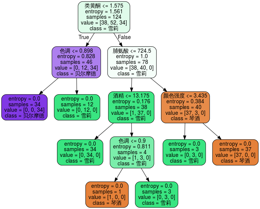
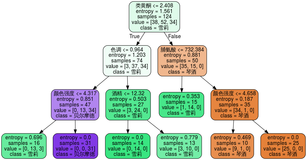
5. 画出决策树

feature_name = ['酒精','苹果酸','灰','灰的碱性','镁','总酚','类黄酮','非黄烷类酚类','花青素','颜色强度','色调','od280/od315稀释葡萄酒','脯氨酸']
class_name = ["琴酒","雪莉","贝尔摩德"]
dot_data = tree.export_graphviz(clf1
                              , feature_names = feature_name
                              , class_names = class_name
                              , filled = True
                              , rounded = True)
graph = graphviz.Source(dot_data)
graph

6. 探索决策树

[*zip(feature_name, clf.feature_importances_)]

[('酒精', 0.0),
 ('苹果酸', 0.034007712273200756),
 ('灰', 0.0),
 ('灰的碱性', 0.03420766509148968),
 ('镁', 0.0),
 ('总酚', 0.0),
 ('类黄酮', 0.4252776947998897),
 ('非黄烷类酚类', 0.0),
 ('花青素', 0.0),
 ('颜色强度', 0.22457026707268818),
 ('色调', 0.0),
 ('od280/od315稀释葡萄酒', 0.0),
 ('脯氨酸', 0.2819366607627316)]

剪枝参数

max_depth
min_samples_leaf
min_samples_split

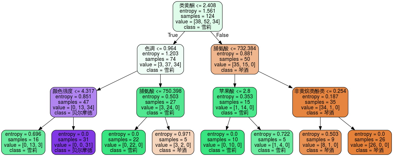
7. 调整参数

clf2 = tree.DecisionTreeClassifier(criterion = 'entropy'
                                  , random_state = 24
                                  , splitter = 'random'
                                 )
clf2.fit(Xtrain, Ytrain)
score = clf2.score(Xtest, Ytest)
score

0.9814814814814815

dot_data = tree.export_graphviz(clf2
                               , feature_names = feature_name
                               , class_names = class_name
                               , filled = True
                               , rounded = True)
graph = graphviz.Source(dot_data)
graph

clf3 = tree.DecisionTreeClassifier(criterion = 'entropy'
                                  , random_state = 24
                                  , splitter = 'random'
                                  , max_depth = 3
                                 )
clf3.fit(Xtrain, Ytrain)
score = clf3.score(Xtest, Ytest)
score

0.9814814814814815

dot_data = tree.export_graphviz(clf3
                               , feature_names = feature_name
                               , class_names = class_name
                               , filled = True
                               , rounded = True)
graph = graphviz.Source(dot_data)
graph

clf4 = tree.DecisionTreeClassifier(criterion = 'entropy'
                                  , random_state = 24
                                  , splitter = 'random'
                                  , max_depth = 3
                                  , min_samples_leaf = 10
                                 )
clf4.fit(Xtrain, Ytrain)
score = clf4.score(Xtest, Ytest)
score

0.9814814814814815

dot_data = tree.export_graphviz(clf4
                               , feature_names = feature_name
                               , class_names = class_name
                               , filled = True
                               , rounded = True)
graph = graphviz.Source(dot_data)
graph

clf5 = tree.DecisionTreeClassifier(criterion = 'entropy'
                                  , random_state = 24
                                  , splitter = 'random'
                                  , max_depth = 3
                                  , min_samples_split = 15
                                 )
clf5.fit(Xtrain, Ytrain)
score = clf5.score(Xtest, Ytest)
score

0.9814814814814815

dot_data = tree.export_graphviz(clf5
                               , feature_names = feature_name
                               , class_names = class_name
                               , filled = True
                               , rounded = True)
graph = graphviz.Source(dot_data)
graph

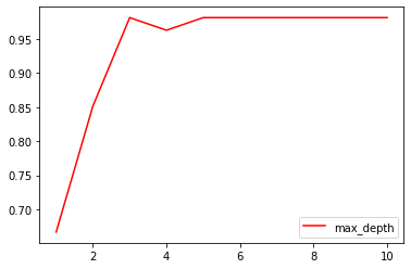
8. 绘制学习曲线，确定最优参数

import matplotlib.pyplot as plt

test = []
for i in range(10):
    clf_best = tree.DecisionTreeClassifier(criterion = 'entropy'
                                  , random_state = 24
                                  , splitter = 'random'
                                  , max_depth = i + 1
                                 )
    clf_best.fit(Xtrain, Ytrain)
    test.append(clf_best.score(Xtest, Ytest))
plt.plot(range(1, 11), test, color = 'r', label = 'max_depth')
plt.legend()

<matplotlib.legend.Legend at 0x21352fec9e8>

# 返回每个测试样本所在的叶子节点的索引
clf5.apply(Xtest)

array([ 4, 13,  4,  6, 13,  4, 14, 14,  4,  6,  4,  3, 14,  6,  4,  4, 14,
       10, 14,  6, 14,  6, 13,  4, 14, 14,  4,  4,  6, 14,  3, 14, 13,  4,
        4, 11,  6, 14, 13, 14, 10,  3, 13,  4, 14,  4, 13, 10,  6,  6, 14,
        3,  6,  4], dtype=int64)

# 返回每个测试样本的分类/回归的结果
clf5.predict(Xtest)

array([2, 0, 2, 1, 0, 2, 0, 0, 2, 1, 2, 1, 0, 1, 2, 2, 0, 1, 0, 1, 0, 1,
       0, 2, 0, 0, 2, 2, 1, 0, 1, 0, 0, 2, 2, 1, 1, 0, 0, 0, 1, 1, 0, 2,
       0, 2, 0, 1, 1, 1, 0, 1, 1, 2])

决策树-回归树

1. 交叉验证cross_val_score的用法

from sklearn.datasets import load_boston
from sklearn.model_selection import cross_val_score
from sklearn.tree import DecisionTreeRegressor

boston = load_boston()
boston

{'data': array([[6.3200e-03, 1.8000e+01, 2.3100e+00, ..., 1.5300e+01, 3.9690e+02,
         4.9800e+00],
        [2.7310e-02, 0.0000e+00, 7.0700e+00, ..., 1.7800e+01, 3.9690e+02,
         9.1400e+00],
        [2.7290e-02, 0.0000e+00, 7.0700e+00, ..., 1.7800e+01, 3.9283e+02,
         4.0300e+00],
        ...,
        [6.0760e-02, 0.0000e+00, 1.1930e+01, ..., 2.1000e+01, 3.9690e+02,
         5.6400e+00],
        [1.0959e-01, 0.0000e+00, 1.1930e+01, ..., 2.1000e+01, 3.9345e+02,
         6.4800e+00],
        [4.7410e-02, 0.0000e+00, 1.1930e+01, ..., 2.1000e+01, 3.9690e+02,
         7.8800e+00]]),
 'target': array([24. , 21.6, 34.7, 33.4, 36.2, 28.7, 22.9, 27.1, 16.5, 18.9, 15. ,
        18.9, 21.7, 20.4, 18.2, 19.9, 23.1, 17.5, 20.2, 18.2, 13.6, 19.6,
        15.2, 14.5, 15.6, 13.9, 16.6, 14.8, 18.4, 21. , 12.7, 14.5, 13.2,
        13.1, 13.5, 18.9, 20. , 21. , 24.7, 30.8, 34.9, 26.6, 25.3, 24.7,
        21.2, 19.3, 20. , 16.6, 14.4, 19.4, 19.7, 20.5, 25. , 23.4, 18.9,
        35.4, 24.7, 31.6, 23.3, 19.6, 18.7, 16. , 22.2, 25. , 33. , 23.5,
        19.4, 22. , 17.4, 20.9, 24.2, 21.7, 22.8, 23.4, 24.1, 21.4, 20. ,
        20.8, 21.2, 20.3, 28. , 23.9, 24.8, 22.9, 23.9, 26.6, 22.5, 22.2,
        23.6, 28.7, 22.6, 22. , 22.9, 25. , 20.6, 28.4, 21.4, 38.7, 43.8,
        33.2, 27.5, 26.5, 18.6, 19.3, 20.1, 19.5, 19.5, 20.4, 19.8, 19.4,
        21.7, 22.8, 18.8, 18.7, 18.5, 18.3, 21.2, 19.2, 20.4, 19.3, 22. ,
        20.3, 20.5, 17.3, 18.8, 21.4, 15.7, 16.2, 18. , 14.3, 19.2, 19.6,
        23. , 18.4, 15.6, 18.1, 17.4, 17.1, 13.3, 17.8, 14. , 14.4, 13.4,
        15.6, 11.8, 13.8, 15.6, 14.6, 17.8, 15.4, 21.5, 19.6, 15.3, 19.4,
        17. , 15.6, 13.1, 41.3, 24.3, 23.3, 27. , 50. , 50. , 50. , 22.7,
        25. , 50. , 23.8, 23.8, 22.3, 17.4, 19.1, 23.1, 23.6, 22.6, 29.4,
        23.2, 24.6, 29.9, 37.2, 39.8, 36.2, 37.9, 32.5, 26.4, 29.6, 50. ,
        32. , 29.8, 34.9, 37. , 30.5, 36.4, 31.1, 29.1, 50. , 33.3, 30.3,
        34.6, 34.9, 32.9, 24.1, 42.3, 48.5, 50. , 22.6, 24.4, 22.5, 24.4,
        20. , 21.7, 19.3, 22.4, 28.1, 23.7, 25. , 23.3, 28.7, 21.5, 23. ,
        26.7, 21.7, 27.5, 30.1, 44.8, 50. , 37.6, 31.6, 46.7, 31.5, 24.3,
        31.7, 41.7, 48.3, 29. , 24. , 25.1, 31.5, 23.7, 23.3, 22. , 20.1,
        22.2, 23.7, 17.6, 18.5, 24.3, 20.5, 24.5, 26.2, 24.4, 24.8, 29.6,
        42.8, 21.9, 20.9, 44. , 50. , 36. , 30.1, 33.8, 43.1, 48.8, 31. ,
        36.5, 22.8, 30.7, 50. , 43.5, 20.7, 21.1, 25.2, 24.4, 35.2, 32.4,
        32. , 33.2, 33.1, 29.1, 35.1, 45.4, 35.4, 46. , 50. , 32.2, 22. ,
        20.1, 23.2, 22.3, 24.8, 28.5, 37.3, 27.9, 23.9, 21.7, 28.6, 27.1,
        20.3, 22.5, 29. , 24.8, 22. , 26.4, 33.1, 36.1, 28.4, 33.4, 28.2,
        22.8, 20.3, 16.1, 22.1, 19.4, 21.6, 23.8, 16.2, 17.8, 19.8, 23.1,
        21. , 23.8, 23.1, 20.4, 18.5, 25. , 24.6, 23. , 22.2, 19.3, 22.6,
        19.8, 17.1, 19.4, 22.2, 20.7, 21.1, 19.5, 18.5, 20.6, 19. , 18.7,
        32.7, 16.5, 23.9, 31.2, 17.5, 17.2, 23.1, 24.5, 26.6, 22.9, 24.1,
        18.6, 30.1, 18.2, 20.6, 17.8, 21.7, 22.7, 22.6, 25. , 19.9, 20.8,
        16.8, 21.9, 27.5, 21.9, 23.1, 50. , 50. , 50. , 50. , 50. , 13.8,
        13.8, 15. , 13.9, 13.3, 13.1, 10.2, 10.4, 10.9, 11.3, 12.3,  8.8,
         7.2, 10.5,  7.4, 10.2, 11.5, 15.1, 23.2,  9.7, 13.8, 12.7, 13.1,
        12.5,  8.5,  5. ,  6.3,  5.6,  7.2, 12.1,  8.3,  8.5,  5. , 11.9,
        27.9, 17.2, 27.5, 15. , 17.2, 17.9, 16.3,  7. ,  7.2,  7.5, 10.4,
         8.8,  8.4, 16.7, 14.2, 20.8, 13.4, 11.7,  8.3, 10.2, 10.9, 11. ,
         9.5, 14.5, 14.1, 16.1, 14.3, 11.7, 13.4,  9.6,  8.7,  8.4, 12.8,
        10.5, 17.1, 18.4, 15.4, 10.8, 11.8, 14.9, 12.6, 14.1, 13. , 13.4,
        15.2, 16.1, 17.8, 14.9, 14.1, 12.7, 13.5, 14.9, 20. , 16.4, 17.7,
        19.5, 20.2, 21.4, 19.9, 19. , 19.1, 19.1, 20.1, 19.9, 19.6, 23.2,
        29.8, 13.8, 13.3, 16.7, 12. , 14.6, 21.4, 23. , 23.7, 25. , 21.8,
        20.6, 21.2, 19.1, 20.6, 15.2,  7. ,  8.1, 13.6, 20.1, 21.8, 24.5,
        23.1, 19.7, 18.3, 21.2, 17.5, 16.8, 22.4, 20.6, 23.9, 22. , 11.9]),
 'feature_names': array(['CRIM', 'ZN', 'INDUS', 'CHAS', 'NOX', 'RM', 'AGE', 'DIS', 'RAD',
        'TAX', 'PTRATIO', 'B', 'LSTAT'], dtype='<U7'),
 'DESCR': ".. _boston_dataset:\n\nBoston house prices dataset\n---------------------------\n\n**Data Set Characteristics:**  \n\n    :Number of Instances: 506 \n\n    :Number of Attributes: 13 numeric/categorical predictive. Median Value (attribute 14) is usually the target.\n\n    :Attribute Information (in order):\n        - CRIM     per capita crime rate by town\n        - ZN       proportion of residential land zoned for lots over 25,000 sq.ft.\n        - INDUS    proportion of non-retail business acres per town\n        - CHAS     Charles River dummy variable (= 1 if tract bounds river; 0 otherwise)\n        - NOX      nitric oxides concentration (parts per 10 million)\n        - RM       average number of rooms per dwelling\n        - AGE      proportion of owner-occupied units built prior to 1940\n        - DIS      weighted distances to five Boston employment centres\n        - RAD      index of accessibility to radial highways\n        - TAX      full-value property-tax rate per $10,000\n        - PTRATIO  pupil-teacher ratio by town\n        - B        1000(Bk - 0.63)^2 where Bk is the proportion of blacks by town\n        - LSTAT    % lower status of the population\n        - MEDV     Median value of owner-occupied homes in $1000's\n\n    :Missing Attribute Values: None\n\n    :Creator: Harrison, D. and Rubinfeld, D.L.\n\nThis is a copy of UCI ML housing dataset.\nhttps://archive.ics.uci.edu/ml/machine-learning-databases/housing/\n\n\nThis dataset was taken from the StatLib library which is maintained at Carnegie Mellon University.\n\nThe Boston house-price data of Harrison, D. and Rubinfeld, D.L. 'Hedonic\nprices and the demand for clean air', J. Environ. Economics & Management,\nvol.5, 81-102, 1978.   Used in Belsley, Kuh & Welsch, 'Regression diagnostics\n...', Wiley, 1980.   N.B. Various transformations are used in the table on\npages 244-261 of the latter.\n\nThe Boston house-price data has been used in many machine learning papers that address regression\nproblems.   \n     \n.. topic:: References\n\n   - Belsley, Kuh & Welsch, 'Regression diagnostics: Identifying Influential Data and Sources of Collinearity', Wiley, 1980. 244-261.\n   - Quinlan,R. (1993). Combining Instance-Based and Model-Based Learning. In Proceedings on the Tenth International Conference of Machine Learning, 236-243, University of Massachusetts, Amherst. Morgan Kaufmann.\n",
 'filename': 'C:\\anaconda\\lib\\site-packages\\sklearn\\datasets\\data\\boston_house_prices.csv'}

regressor = DecisionTreeRegressor(random_state = 0)
cross_val_score(regressor, boston.data, boston.target, cv = 10,
                scoring = 'neg_mean_squared_error')

array([-16.41568627, -10.61843137, -18.30176471, -55.36803922,
       -16.01470588, -44.70117647, -12.2148    , -91.3888    ,
       -57.764     , -36.8134    ])

2. 一维回归图像的绘制

import numpy as np

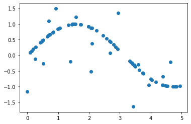
创建一条含噪声的正弦曲线

rng = np.random.RandomState(1) # 随机数种子
x = np.sort(5 * rng.rand(80, 1), # 80行1列，二维数组
            axis = 0)
# np.random.rand(数组结构)
y = np.sin(x).ravel() # 将y降为一维，一维数组不分行列
y[::5] += 3 * (0.5 - rng.rand(16)) # 在正弦曲线上增加正负1.5之间的噪声，因为训练集是对不可得的全集的抽样

降维函数ravel()的用法：

将n维数组降成n-1维，多次运行可以降到一维为止 np.random.random((2, 1)) np.random.random((2, 1)).ravel()

np.random.random((2, 1))

array([[0.03439227],
       [0.02179519]])

np.random.random((2, 1)).ravel()

array([0.08286905, 0.32139659])

np.random.random((2, 1)).ravel().shape

(2,)

plt.scatter(x, y, label)

<matplotlib.collections.PathCollection at 0x21353138748>

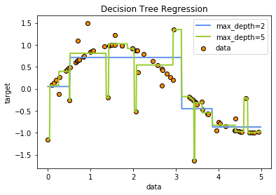
实例化 & 训练模型

regression1 = DecisionTreeRegressor(max_depth = 2)
regression2 = DecisionTreeRegressor(max_depth = 5)
regression1.fit(x, y)
regression2.fit(x, y)

DecisionTreeRegressor(criterion='mse', max_depth=5, max_features=None,
                      max_leaf_nodes=None, min_impurity_decrease=0.0,
                      min_impurity_split=None, min_samples_leaf=1,
                      min_samples_split=2, min_weight_fraction_leaf=0.0,
                      presort=False, random_state=None, splitter='best')

创建测试集

x_test = np.arange(0.0, 5.0, 0.01) # 生成序列，参数依次为开始点、结束点、步长
x_test[:10]

array([0.  , 0.01, 0.02, 0.03, 0.04, 0.05, 0.06, 0.07, 0.08, 0.09])

x_test = x_test[:, np.newaxis]

增维的几种方法，以np.array([1, 2, 3, 4])为例：

增维切片np.newaxis的用法： np.array([1, 2, 3, 4])[:, np.newaxis] np.array([1, 2, 3, 4])[np.newaxis, :]

newaxis = None： np.array([1, 2, 3, 4])[:, None] np.array([1, 2, 3, 4])[None, :]

方法.reshape()的用法： np.array([1, 2, 3, 4]).reshape(-1, 1) np.array([1, 2, 3, 4]).reshape(1, -1)

np.array([1, 2, 3, 4])

array([1, 2, 3, 4])

np.array([1, 2, 3, 4])[:, np.newaxis]

array([[1],
       [2],
       [3],
       [4]])

np.array([1, 2, 3, 4])[np.newaxis, :]

array([[1, 2, 3, 4]])

np.array([1, 2, 3, 4])[:, None]

array([[1],
       [2],
       [3],
       [4]])

np.array([1, 2, 3, 4])[None, :]

array([[1, 2, 3, 4]])

np.array([1, 2, 3, 4]).reshape(-1, 1)

array([[1],
       [2],
       [3],
       [4]])

np.array([1, 2, 3, 4]).reshape(1, -1)

array([[1, 2, 3, 4]])

测试集导入模型，预测结果

y1 = regression1.predict(x_test)
y2 = regression2.predict(x_test)

绘制图像

plt.figure()
plt.scatter(x, y, edgecolor = 'black', c = 'darkorange', label = 'data')
plt.plot(x_test, y1, color = 'cornflowerblue', label = 'max_depth=2', linewidth = 2)
plt.plot(x_test, y2, color = 'yellowgreen', label = 'max_depth=5', linewidth = 2)
plt.xlabel('data')
plt.ylabel('target')
plt.title('Decision Tree Regression')
plt.legend()

<matplotlib.legend.Legend at 0x21353101940>

二、泰坦尼克号生存预测

import numpy as np
import pandas as pd
import matplotlib.pyplot as plt
from sklearn.tree import DecisionTreeClassifier
from sklearn.model_selection import GridSearchCV
from sklearn.model_selection import train_test_split

1. 导入数据集 & 数据预处理

data = pd.read_csv('data.csv')

探索数据

data.head()

	PassengerId	Survived	Pclass	Name	Sex	Age	SibSp	Ticket	Fare	Cabin	Embarked
0	1	0	3	Braund, Mr. Owen Harris	male	22.0	1	A/5 21171	7.2500	NaN	S
1	2	1	1	Cumings, Mrs. John Bradley (Florence Briggs Th…	female	38.0	1	PC 17599	71.2833	C85	C
2	3	1	3	Heikkinen, Miss. Laina	female	26.0	0	STON/O2. 3101282	7.9250	NaN	S
3	4	1	1	Futrelle, Mrs. Jacques Heath (Lily May Peel)	female	35.0	1	113803	53.1000	C123	S
4	5	0	3	Allen, Mr. William Henry	male	35.0	0	373450	8.0500	NaN	S

该数据集的标签为’Survived’

data.info()

<class 'pandas.core.frame.DataFrame'>
RangeIndex: 891 entries, 0 to 890
Data columns (total 12 columns):
PassengerId    891 non-null int64
Survived       891 non-null int64
Pclass         891 non-null int64
Name           891 non-null object
Sex            891 non-null object
Age            714 non-null float64
SibSp          891 non-null int64
Parch          891 non-null int64
Ticket         891 non-null object
Fare           891 non-null float64
Cabin          204 non-null object
Embarked       889 non-null object
dtypes: float64(2), int64(5), object(5)
memory usage: 83.6+ KB

关于分类的文本信息需要被转换为数字
处理缺失值
处理无用特征

data.describe()

	PassengerId	Survived	Pclass	Age	SibSp	Parch	Fare
count	891.000000	891.000000	891.000000	714.000000	891.000000	891.000000	891.000000
mean	446.000000	0.383838	2.308642	29.699118	0.523008	0.381594	32.204208
std	257.353842	0.486592	0.836071	14.526497	1.102743	0.806057	49.693429
min	1.000000	0.000000	1.000000	0.420000	0.000000	0.000000	0.000000
25%	223.500000	0.000000	2.000000	20.125000	0.000000	0.000000	7.910400
50%	446.000000	0.000000	3.000000	28.000000	0.000000	0.000000	14.454200
75%	668.500000	1.000000	3.000000	38.000000	1.000000	0.000000	31.000000
max	891.000000	1.000000	3.000000	80.000000	8.000000	6.000000	512.329200

# 筛选特征
data.drop(['Name', 'Ticket', 'Cabin'], # Cabin缺失太多
          inplace = True, axis = 1)
# 处理缺失值：填补
data.loc[:, 'Age'].fillna(data.loc[:, 'Age'].mean(), inplace = True) # 不是所有数值型变量都可以用均值填补，但是年龄特征在填补数量不大的情况下进行填补，是可以接受的
# 也可以用随机森林进行填补
# 处理缺失值：删除
data.dropna(axis = 0)
# 将二分类变量转换为数值型变量
data.loc[:, 'Sex'] = (data.loc[:, 'Sex'] == 'male').astype('int')
# 将三分类变量转换为数值型变量
labels = data.loc[:, 'Embarked'].unique().tolist()
data.loc[:, 'Embarked'] = data.loc[:, 'Embarked'].apply(lambda x : labels.index(x))

data.head()

	PassengerId	Survived	Pclass	Sex	Age	SibSp	Fare	Embarked
0	1	0	3	1	22.0	1	7.2500	0
1	2	1	1	0	38.0	1	71.2833	1
2	3	1	3	0	26.0	0	7.9250	0
3	4	1	1	0	35.0	1	53.1000	0
4	5	0	3	1	35.0	0	8.0500	0

data.info()

<class 'pandas.core.frame.DataFrame'>
RangeIndex: 891 entries, 0 to 890
Data columns (total 9 columns):
PassengerId    891 non-null int64
Survived       891 non-null int64
Pclass         891 non-null int64
Sex            891 non-null int32
Age            891 non-null float64
SibSp          891 non-null int64
Parch          891 non-null int64
Fare           891 non-null float64
Embarked       891 non-null int64
dtypes: float64(2), int32(1), int64(6)
memory usage: 59.2 KB

2. 提取标签和特征矩阵，分测试集和训练集

x = data.loc[:, data.columns[data.columns != 'Survived']]

x.head()

	PassengerId	Pclass	Sex	Age	SibSp	Fare	Embarked
0	1	3	1	22.0	1	7.2500	0
1	2	1	0	38.0	1	71.2833	1
2	3	3	0	26.0	0	7.9250	0
3	4	1	0	35.0	1	53.1000	0
4	5	3	1	35.0	0	8.0500	0

x = data.iloc[:, data.columns != 'Survived']

x.head()

	PassengerId	Pclass	Sex	Age	SibSp	Fare	Embarked
0	1	3	1	22.0	1	7.2500	0
1	2	1	0	38.0	1	71.2833	1
2	3	3	0	26.0	0	7.9250	0
3	4	1	0	35.0	1	53.1000	0
4	5	3	1	35.0	0	8.0500	0

y = data.loc[:, 'Survived']
y.head()

0    0
1    1
2    1
3    1
4    0
Name: Survived, dtype: int64

y = data.loc[:, data.columns == 'Survived']
y.head()

	Survived
0	0
1	1
2	1
3	1
4	0

Xtrain, Xtest, Ytrain, Ytest = train_test_split(x, y, test_size = 0.3)

Xtrain.head()

	PassengerId	Pclass	Sex	Age	SibSp	Fare	Embarked
430	431	1	1	28.0	0	26.5500	0
39	40	3	0	14.0	1	11.2417	1
290	291	1	0	26.0	0	78.8500	0
875	876	3	0	15.0	0	7.2250	1
89	90	3	1	24.0	0	8.0500	0

纠正索引

for i in [Xtrain, Xtest, Ytrain, Ytest]:
    i.index = range(i.shape[0])

Xtrain.head()

	PassengerId	Pclass	Sex	Age	SibSp	Fare	Embarked
0	431	1	1	28.0	0	26.5500	0
1	40	3	0	14.0	1	11.2417	1
2	291	1	0	26.0	0	78.8500	0
3	876	3	0	15.0	0	7.2250	1
4	90	3	1	24.0	0	8.0500	0

3. 导入模型

clf = DecisionTreeClassifier(random_state = 25)
clf.fit(Xtrain, Ytrain)
score = clf.score(Xtest, Ytest)

score

0.7313432835820896

clf = DecisionTreeClassifier(random_state = 25)
score = cross_val_score(clf, x, y, cv = 10).mean()
score

0.7532036658722052

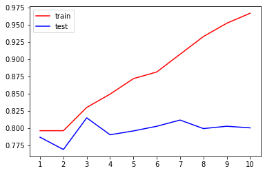
4. 在不同max_depth下观察模型的拟合情况

train = []
test = []
for i in range(10):
    clf = DecisionTreeClassifier(random_state = 25, max_depth = i + 1)
    clf.fit(Xtrain, Ytrain)
    score_train = clf.score(Xtrain, Ytrain)
    score_test = cross_val_score(clf, x, y, cv = 10).mean()
    train.append(score_train)
    test.append(score_test)
plt.figure()
plt.plot(range(1, 11), train, color = 'red', label = 'train')
plt.plot(range(1, 11), test, color = 'blue', label = 'test')
plt.xticks(range(1, 11))
plt.legend()
max(test)

0.8147891839745773

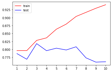
train = []
test = []
for i in range(10):
    clf = DecisionTreeClassifier(random_state = 25, max_depth = i + 1, criterion = 'entropy') # 在模型欠拟合时使用entropy
    clf.fit(Xtrain, Ytrain)
    score_train = clf.score(Xtrain, Ytrain)
    score_test = cross_val_score(clf, x, y, cv = 10).mean()
    train.append(score_train)
    test.append(score_test)
plt.figure()
plt.plot(range(1, 11), train, color = 'red', label = 'train')
plt.plot(range(1, 11), test, color = 'blue', label = 'test')
plt.xticks(range(1, 11))
plt.legend()
max(test)

0.8181730223584156

5. 用网格搜索调整参数

# entropy_threholds = np.linspace(0, 1, 20) 信息增益边界
# gini_threholds = np.linspace(0, 0.5, 20) 基尼系数边界
# 网格搜索里的参数：
# 1. 一串参数
# 2. 这些参数对应的，我们希望网格搜索来搜索的参数的取值范围
parameters = {'criterion':('gini', 'entropy')
            , 'splitter':('best', 'random')
            , 'max_depth':[*range(1, 10)]
            , 'min_samples_leaf':[*range(1, 50, 5)] 
            , 'min_impurity_decrease':np.linspace(0, 1, 20)
             }
clf = DecisionTreeClassifier(random_state = 25)
GS = GridSearchCV(clf, parameters, cv = 10)
# 同时实现fit、score和cross_val_score
GS.fit(Xtrain, Ytrain)

C:\anaconda\lib\site-packages\sklearn\model_selection\_search.py:813: DeprecationWarning: The default of the `iid` parameter will change from True to False in version 0.22 and will be removed in 0.24. This will change numeric results when test-set sizes are unequal.
  DeprecationWarning)
GridSearchCV(cv=10, error_score='raise-deprecating',
             estimator=DecisionTreeClassifier(class_weight=None,
                                              criterion='gini', max_depth=None,
                                              max_features=None,
                                              max_leaf_nodes=None,
                                              min_impurity_decrease=0.0,
                                              min_impurity_split=None,
                                              min_samples_leaf=1,
                                              min_samples_split=2,
                                              min_weight_fraction_leaf=0.0,
                                              presort=False, random_state=25,
                                              splitter='best'),
             iid='warn', n_...
                         'min_impurity_decrease': array([0.        , 0.05263158, 0.10526316, 0.15789474, 0.21052632,
       0.26315789, 0.31578947, 0.36842105, 0.42105263, 0.47368421,
       0.52631579, 0.57894737, 0.63157895, 0.68421053, 0.73684211,
       0.78947368, 0.84210526, 0.89473684, 0.94736842, 1.        ]),
                         'min_samples_leaf': [1, 6, 11, 16, 21, 26, 31, 36, 41,
                                              46],
                         'splitter': ('best', 'random')},
             pre_dispatch='2*n_jobs', refit=True, return_train_score=False,
             scoring=None, verbose=0)

GS.best_params_ # 从我们输入的参数和参数取值列表中，返回最佳的组合

{'criterion': 'gini',
 'max_depth': 4,
 'min_impurity_decrease': 0.0,
 'min_samples_leaf': 26,
 'splitter': 'random'}

GS.best_score_ # 网格搜索后的模型的评判标准
# 因为现在是分类模型，所以score是在最佳参数组合下的accuracy

0.8170144462279294

clf = DecisionTreeClassifier(random_state = 25, criterion = 'gini', 
                             max_depth = 4, min_samples_leaf = 26, 
                             splitter = 'random')
clf.fit(Xtrain, Ytrain)
clf.score(Xtest, Ytest)

0.8171641791044776

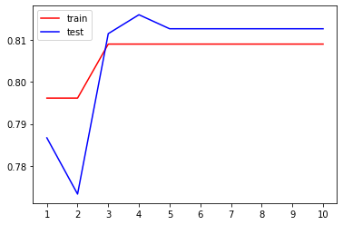
train = []
test = []
for i in range(10):
    clf = DecisionTreeClassifier(random_state = 25, criterion = 'gini', 
                                 max_depth = i + 1, min_samples_leaf = 26, 
                                 splitter = 'random')
    clf.fit(Xtrain, Ytrain)
    score_train = clf.score(Xtrain, Ytrain)
    score_test = cross_val_score(clf, x, y, cv = 10).mean()
    train.append(score_train)
    test.append(score_test)
plt.figure()
plt.plot(range(1, 11), train, color = 'red', label = 'train')
plt.plot(range(1, 11), test, color = 'blue', label = 'test')
plt.xticks(range(1, 11))
plt.legend()
max(test)

0.8159627170582228

决策树与泰坦尼克号生存预测

一、 决策树