一、 逻辑回归概述
from sklearn.linear_model import LogisticRegression as LRfrom sklearn.datasets import load_breast_cancerimport numpy as npimport pandas as pdimport matplotlib.pyplot as plt%matplotlib inlinefrom sklearn.model_selection import train_test_splitfrom sklearn.metrics import accuracy_scorefrom sklearn.model_selection import cross_val_scorefrom sklearn.feature_selection import SelectFromModel
data = load_breast_cancer() # 实例化,得到一个字典x = data.datay = data.targetx.shape
(569, 30)
lrl1 = LR(penalty = 'l1', solver = 'liblinear', C = 0.5, max_iter = 1000)lrl2 = LR(penalty = 'l2', solver = 'liblinear', C = 0.5, max_iter = 1000)
lrl1 = lrl1.fit(x, y)lrl1.coef_
array([[ 3.99870273, 0.03177392, -0.13689412, -0.01621641, 0. ,0. , 0. , 0. , 0. , 0. ,0. , 0.50497324, 0. , -0.07127604, 0. ,0. , 0. , 0. , 0. , 0. ,0. , -0.24570638, -0.12849964, -0.01441515, 0. ,0. , -2.04390881, 0. , 0. , 0. ]])
(lrl1.coef_ != 0).sum(axis = 1)
array([10])
lrl2 = lrl2.fit(x, y)lrl2.coef_
array([[ 1.61543234e+00, 1.02284415e-01, 4.78483684e-02,-4.43927107e-03, -9.42247882e-02, -3.01420673e-01,-4.56065677e-01, -2.22346063e-01, -1.35660484e-01,-1.93917198e-02, 1.61646580e-02, 8.84531037e-01,1.20301273e-01, -9.47422278e-02, -9.81687769e-03,-2.37399092e-02, -5.71846204e-02, -2.70190106e-02,-2.77563737e-02, 1.98122260e-04, 1.26394730e+00,-3.01762592e-01, -1.72784162e-01, -2.21786411e-02,-1.73339657e-01, -8.79070550e-01, -1.16325561e+00,-4.27661014e-01, -4.20612369e-01, -8.69820058e-02]])
L1正则化本质上是一种特征选择
L2正则化在加强的过程中,会尽量让每一个特征都对模型有贡献
l1 = []l2 = []l1test = []l2test = []Xtrain, Xtest, Ytrain, Ytest = train_test_split(x, y, test_size = 0.3, random_state = 420)for i in np.linspace(0.05, 1, 19):lrl1 = LR(C = i, penalty = 'l1', solver = 'liblinear', max_iter = 1000)lrl2 = LR(C = i, penalty = 'l2', solver = 'liblinear', max_iter = 1000)lrl1.fit(Xtrain, Ytrain)lrl2.fit(Xtrain, Ytrain)l1.append(accuracy_score(lrl1.predict(Xtrain), Ytrain))l1test.append(accuracy_score(lrl1.predict(Xtest), Ytest))l2.append(accuracy_score(lrl2.predict(Xtrain), Ytrain))l2test.append(accuracy_score(lrl2.predict(Xtest), Ytest))plt.figure(figsize = (6, 6))graph = [l1, l2, l1test, l2test]color = ['green', 'black', 'lightgreen', 'gray']label = ['L1', 'L2', 'L1test', 'L2test']for i in range(len(graph)):plt.plot(np.linspace(0.05, 1, 19), graph[i], color = color[i], label = label[i])plt.legend()
<matplotlib.legend.Legend at 0x1eb56390278>
逻辑回归在训练时的目标是,提高训练集的预测准确率。所以这里监控训练集的准确率。
二、 逻辑回归的特征工程
- 业务选择
- PCA 和 SVD
- 统计方法
- 嵌入法 Embedded
LR_ = LR(solver = 'liblinear', C = 0.8, random_state = 420)cross_val_score(LR_, x, y, cv = 10).mean()
0.9508145363408522
x_embedded = SelectFromModel(LR_,norm_order = 1 # 使用L1范式筛选,模型会去掉所有在L1范式下被判断为无效的特征).fit_transform(x, y)x_embedded.shape
(569, 9)
x.shape
(569, 30)
cross_val_score(LR_, x_embedded, y).mean()
0.9349945660611707
进一步提升模型的拟合效果
1. 调节threshold
根据特征重要性选择特征
在逻辑回归中,特征重要性就是系数,此时特征选择的判断指标就不是L1范数,而是属性coef_,即特征的参数
abs(LR_.fit(x, y).coef_).max()
1.9407192479360273
LR_.fit(x, y).coef_
array([[ 1.94071925, 0.11027501, -0.02792478, -0.00347267, -0.13418458,-0.36887791, -0.58229351, -0.30118379, -0.19522369, -0.02391175,-0.01172073, 1.12398531, 0.04214842, -0.0940855 , -0.01457835,-0.00486005, -0.05146662, -0.03584081, -0.03757288, 0.0042326 ,1.24863871, -0.32757391, -0.13662037, -0.0236736 , -0.24820117,-1.05186104, -1.44596614, -0.57989786, -0.6022902 , -0.10544953]])
系数越大,该系数对应的特征对逻辑回归贡献越大
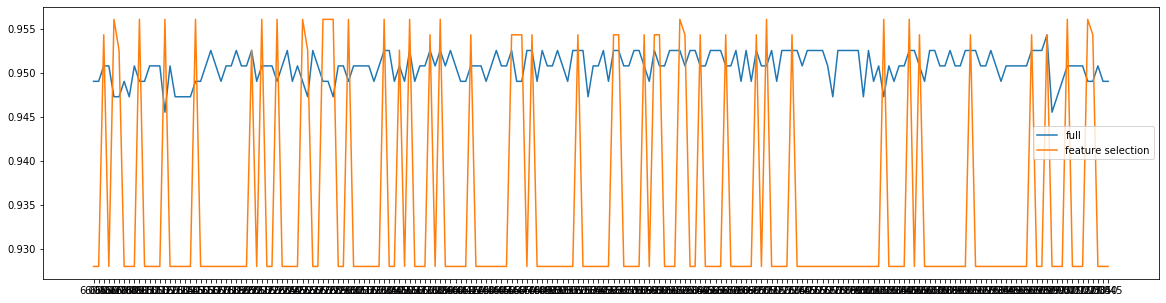
fullx = []fsx = []threshold = np.linspace(0, abs(LR_.fit(x, y).coef_).max(), 20)k = 0for i in threshold:x_embedded = SelectFromModel(LR_, threshold = i).fit_transform(x, y)fullx.append(cross_val_score(LR_, x, y, cv = 5).mean())fsx.append(cross_val_score(LR_, x_embedded, y, cv = 5).mean())print(threshold[k], x_embedded.shape[1])k += 1plt.figure(figsize = (20, 5))plt.plot(threshold, fullx, label = 'full')plt.plot(threshold, fsx, label = 'feature selection')plt.xticks(threshold)plt.legend()
0.0 300.1021431183124225 170.204286236624845 120.3064293549372675 100.40857247324969 80.5107155915621124 80.612858709874535 50.7150018281869575 50.81714494649938 50.9192880648118025 51.0214311831242249 51.1235743014366475 41.22571741974907 31.3278605380614925 21.430003656373915 21.5321467746863375 11.63428989299876 11.7364330113111823 11.838576129623605 11.9407192479360273 1<matplotlib.legend.Legend at 0x1eb56460780>
细化学习曲线
fullx = []fsx = []threshold = np.linspace(0, 0.1021431183124225, 20)k = 0for i in threshold:x_embedded = SelectFromModel(LR_, threshold = i).fit_transform(x, y)fullx.append(cross_val_score(LR_, x, y, cv = 5).mean())fsx.append(cross_val_score(LR_, x_embedded, y, cv = 5).mean())print(threshold[k], x_embedded.shape[1])k += 1plt.figure(figsize = (20, 5))plt.plot(threshold, fullx, label = 'full')plt.plot(threshold, fsx, label = 'feature selection')plt.xticks(threshold)plt.legend()
0.0 300.005375953595390658 270.010751907190781316 270.016127860786171976 250.021503814381562632 250.026879767976953288 230.03225572157234395 220.03763167516773461 200.043007628763125264 190.04838358235851592 190.053759535953906576 180.05913548954929724 180.0645114431446879 180.06988739674007856 180.07526335033546921 180.08063930393085987 180.08601525752625053 180.09139121112164118 180.09676716471703184 170.1021431183124225 17<matplotlib.legend.Legend at 0x1eb566f7c88>
要想保持较高的准确率,仍需25个特征。因此调节threshold属于无效的方法。
2. 调节逻辑回归的类LR
使用L1范数,通过画C的学习曲线来实现
fullx = []fsx = []C = np.arange(0.01, 10.01, 0.5)for i in C:LR_ = LR(solver = 'liblinear', C = i, random_state = 420) # 因为时调节模型本身,所以每次循环都需要重新建模x_embedded = SelectFromModel(LR_, norm_order = 1).fit_transform(x, y)fullx.append(cross_val_score(LR_, x, y, cv = 10).mean())fsx.append(cross_val_score(LR_, x_embedded, y, cv = 10).mean())print(max(fsx), C[fsx.index(max(fsx))])plt.figure(figsize = (20, 5))plt.plot(C, fullx, label = 'full')plt.plot(C, fsx, label = 'feature selection')plt.xticks(C)plt.legend()
0.9561090225563911 7.01<matplotlib.legend.Legend at 0x1eb56890f28>
特征选择后,模型效果波动较大,数次好于特征选择前的模型效果
细化学习曲线
fullx = []fsx = []C = np.arange(6.05, 7.05, 0.005)for i in C:LR_ = LR(solver = 'liblinear', C = i, random_state = 420) # 因为时调节模型本身,所以每次循环都需要重新建模x_embedded = SelectFromModel(LR_, norm_order = 1).fit_transform(x, y)fullx.append(cross_val_score(LR_, x, y, cv = 10).mean())fsx.append(cross_val_score(LR_, x_embedded, y, cv = 10).mean())print(max(fsx), C[fsx.index(max(fsx))])plt.figure(figsize = (20, 5))plt.plot(C, fullx, label = 'full')plt.plot(C, fsx, label = 'feature selection')plt.xticks(C)plt.legend()
0.9561090225563911 6.069999999999999<matplotlib.legend.Legend at 0x1eb56b13978>
LR_ = LR(solver = 'liblinear', C = 6.069999999999999, random_state = 420)cross_val_score(LR_, x, y, cv = 10).mean()
0.9473057644110275
LR_ = LR(solver = 'liblinear', C = 6.069999999999999, random_state = 420)x_embedded = SelectFromModel(LR_, norm_order = 1).fit_transform(x, y)cross_val_score(LR_, x_embedded, y, cv = 10).mean()
0.9561090225563911
x_embedded.shape
(569, 11)
- 系数累加法
- 包装法
三、 重要参数及概念
参数
max_iter multi_class ovr: one-vs-rest 表示分类问题是二分类,或让模型使用“一对多”的形式来处理问。0.21版本的默认值
multinomial: many-vs-many 表示处理多分类问题。这种输入在参数solve是’liblinear’时不可用
auto 根据数据的分类情况和其他参数,来确定模型要处理的分类问题的类型 如果数据是二分类,或solver取值为’liblinear’,’auto’默认选择’ovr’ 反之,则会选择’multinomial’
solver
- liblinear:坐标下降法,二分类和ovr专用
- lbfgs
- newton-cg
- sag:随机平均梯度下降,与普通梯度下降法的区别是每次迭代仅用一部分的样本来计算梯度
- saga:随机平均梯度下降,用来处理稀疏多项逻辑回归
class_weight
概念
梯度
>
步长
步长不是任何物理距离,它甚至不是梯度下降过程中任何距离的直接变化,它是梯度向量的大小d上的一个比例,影响着参数向量
每次迭代后改变的部分
样本不均衡
- 标签的一类天然占有很大的比例
- 误分类的代价很高
以上两种状况下,我们希望准确捕获少数类,甚至不惜误判多数类 给占比小的标签更多的权重,让模型往偏向少数类的方向建模
解决方法
- 调节参数class_weight
- 采样法
上采样:增加少数类的样本 下采样:减少多数类的样本

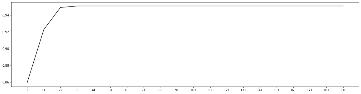
l2 = []Xtrain, Xtest, Ytrain, Ytest = train_test_split(x, y)for i in range(1, 201, 10):lrl2 = LR(penalty = 'l2', solver = 'liblinear', C = 0.8, max_iter = i)lrl2.fit(Xtrain, Ytrain)l2.append(cross_val_score(lrl2, x, y).mean())plt.figure(figsize = (20, 5))plt.plot(range(1, 201, 10), l2, 'black')plt.xticks(range(1, 201, 10));
C:\anaconda\lib\site-packages\sklearn\svm\_base.py:947: ConvergenceWarning: Liblinear failed to converge, increase the number of iterations."the number of iterations.", ConvergenceWarning)C:\anaconda\lib\site-packages\sklearn\svm\_base.py:947: ConvergenceWarning: Liblinear failed to converge, increase the number of iterations."the number of iterations.", ConvergenceWarning)C:\anaconda\lib\site-packages\sklearn\svm\_base.py:947: ConvergenceWarning: Liblinear failed to converge, increase the number of iterations."the number of iterations.", ConvergenceWarning)C:\anaconda\lib\site-packages\sklearn\svm\_base.py:947: ConvergenceWarning: Liblinear failed to converge, increase the number of iterations."the number of iterations.", ConvergenceWarning)C:\anaconda\lib\site-packages\sklearn\svm\_base.py:947: ConvergenceWarning: Liblinear failed to converge, increase the number of iterations."the number of iterations.", ConvergenceWarning)C:\anaconda\lib\site-packages\sklearn\svm\_base.py:947: ConvergenceWarning: Liblinear failed to converge, increase the number of iterations."the number of iterations.", ConvergenceWarning)C:\anaconda\lib\site-packages\sklearn\svm\_base.py:947: ConvergenceWarning: Liblinear failed to converge, increase the number of iterations."the number of iterations.", ConvergenceWarning)C:\anaconda\lib\site-packages\sklearn\svm\_base.py:947: ConvergenceWarning: Liblinear failed to converge, increase the number of iterations."the number of iterations.", ConvergenceWarning)C:\anaconda\lib\site-packages\sklearn\svm\_base.py:947: ConvergenceWarning: Liblinear failed to converge, increase the number of iterations."the number of iterations.", ConvergenceWarning)C:\anaconda\lib\site-packages\sklearn\svm\_base.py:947: ConvergenceWarning: Liblinear failed to converge, increase the number of iterations."the number of iterations.", ConvergenceWarning)C:\anaconda\lib\site-packages\sklearn\svm\_base.py:947: ConvergenceWarning: Liblinear failed to converge, increase the number of iterations."the number of iterations.", ConvergenceWarning)C:\anaconda\lib\site-packages\sklearn\svm\_base.py:947: ConvergenceWarning: Liblinear failed to converge, increase the number of iterations."the number of iterations.", ConvergenceWarning)C:\anaconda\lib\site-packages\sklearn\svm\_base.py:947: ConvergenceWarning: Liblinear failed to converge, increase the number of iterations."the number of iterations.", ConvergenceWarning)C:\anaconda\lib\site-packages\sklearn\svm\_base.py:947: ConvergenceWarning: Liblinear failed to converge, increase the number of iterations."the number of iterations.", ConvergenceWarning)C:\anaconda\lib\site-packages\sklearn\svm\_base.py:947: ConvergenceWarning: Liblinear failed to converge, increase the number of iterations."the number of iterations.", ConvergenceWarning)C:\anaconda\lib\site-packages\sklearn\svm\_base.py:947: ConvergenceWarning: Liblinear failed to converge, increase the number of iterations."the number of iterations.", ConvergenceWarning)C:\anaconda\lib\site-packages\sklearn\svm\_base.py:947: ConvergenceWarning: Liblinear failed to converge, increase the number of iterations."the number of iterations.", ConvergenceWarning)
l2 = []l2test = []Xtrain, Xtest, Ytrain, Ytest = train_test_split(x, y, test_size = 0.3, random_state = 420)for i in range(1, 201, 10):lrl2 = LR(penalty = 'l2', solver = 'liblinear', C = 0.8, max_iter = i)lrl2.fit(Xtrain, Ytrain)l2.append(accuracy_score(lrl2.predict(Xtrain), Ytrain))l2test.append(accuracy_score(lrl2.predict(Xtest), Ytest))graph = [l2, l2test]label = ['l2', 'l2test']color = ['black', 'gray']plt.figure(figsize = (20, 5))for i in range(len(graph)):plt.plot(range(1, 201, 10), graph[i], color = color[i], label = label[i])plt.legend()plt.xticks(range(1, 201, 10));
C:\anaconda\lib\site-packages\sklearn\svm\_base.py:947: ConvergenceWarning: Liblinear failed to converge, increase the number of iterations."the number of iterations.", ConvergenceWarning)C:\anaconda\lib\site-packages\sklearn\svm\_base.py:947: ConvergenceWarning: Liblinear failed to converge, increase the number of iterations."the number of iterations.", ConvergenceWarning)C:\anaconda\lib\site-packages\sklearn\svm\_base.py:947: ConvergenceWarning: Liblinear failed to converge, increase the number of iterations."the number of iterations.", ConvergenceWarning)
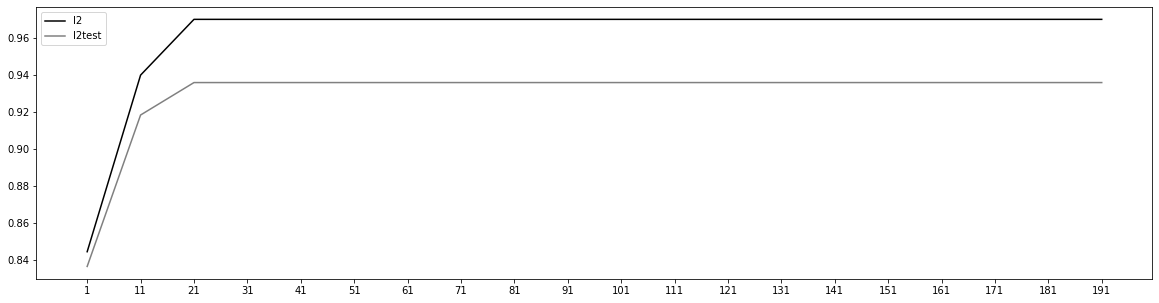
lrl2.n_iter_
array([24], dtype=int32)
from sklearn.datasets import load_irisiris = load_iris()
set(iris.target)
{0, 1, 2}
for multi_class in ('multinomial', 'ovr'):lr = LR(solver = 'sag', max_iter = 100, random_state = 42,multi_class = multi_class).fit(iris.data, iris.target)print('training score: %.3f (%s)' % (lr.score(iris.data, iris.target), multi_class))
training score: 0.987 (multinomial)training score: 0.960 (ovr)C:\anaconda\lib\site-packages\sklearn\linear_model\_sag.py:330: ConvergenceWarning: The max_iter was reached which means the coef_ did not converge"the coef_ did not converge", ConvergenceWarning)C:\anaconda\lib\site-packages\sklearn\linear_model\_sag.py:330: ConvergenceWarning: The max_iter was reached which means the coef_ did not converge"the coef_ did not converge", ConvergenceWarning)C:\anaconda\lib\site-packages\sklearn\linear_model\_sag.py:330: ConvergenceWarning: The max_iter was reached which means the coef_ did not converge"the coef_ did not converge", ConvergenceWarning)C:\anaconda\lib\site-packages\sklearn\linear_model\_sag.py:330: ConvergenceWarning: The max_iter was reached which means the coef_ did not converge"the coef_ did not converge", ConvergenceWarning)
y_predict = lr.predict(iris.data)y_predict
array([0, 0, 0, 0, 0, 0, 0, 0, 0, 0, 0, 0, 0, 0, 0, 0, 0, 0, 0, 0, 0, 0,0, 0, 0, 0, 0, 0, 0, 0, 0, 0, 0, 0, 0, 0, 0, 0, 0, 0, 0, 0, 0, 0,0, 0, 0, 0, 0, 0, 1, 1, 1, 1, 1, 1, 1, 1, 1, 1, 1, 1, 1, 1, 1, 1,2, 1, 1, 1, 2, 1, 1, 1, 1, 1, 1, 2, 1, 1, 1, 1, 1, 2, 2, 2, 1, 1,1, 1, 1, 1, 1, 1, 1, 1, 1, 1, 1, 1, 2, 2, 2, 2, 2, 2, 2, 2, 2, 2,2, 2, 2, 2, 2, 2, 2, 2, 2, 2, 2, 2, 2, 2, 2, 2, 2, 2, 2, 2, 2, 2,2, 2, 2, 2, 2, 2, 2, 2, 2, 2, 2, 2, 2, 2, 2, 2, 2, 2])
(y_predict == iris.target).sum()/len(iris.target)
0.96
四、 案例:评分卡
数据预处理
data = pd.read_csv('rankingcard.csv', index_col = 0)
data.head()
| SeriousDlqin2yrs | RevolvingUtilizationOfUnsecuredLines | age | NumberOfTime30-59DaysPastDueNotWorse | DebtRatio | MonthlyIncome | NumberOfOpenCreditLinesAndLoans | NumberOfTimes90DaysLate | NumberRealEstateLoansOrLines | NumberOfTime60-89DaysPastDueNotWorse | NumberOfDependents | |
|---|---|---|---|---|---|---|---|---|---|---|---|
| 1 | 1 | 0.766127 | 45 | 2 | 0.802982 | 9120.0 | 13 | 0 | 6 | 0 | 2.0 |
| 2 | 0 | 0.957151 | 40 | 0 | 0.121876 | 2600.0 | 4 | 0 | 0 | 0 | 1.0 |
| 3 | 0 | 0.658180 | 38 | 1 | 0.085113 | 3042.0 | 2 | 1 | 0 | 0 | 0.0 |
| 4 | 0 | 0.233810 | 30 | 0 | 0.036050 | 3300.0 | 5 | 0 | 0 | 0 | 0.0 |
| 5 | 0 | 0.907239 | 49 | 1 | 0.024926 | 63588.0 | 7 | 0 | 1 | 0 | 0.0 |
data.shape
(150000, 11)
data.info()
<class 'pandas.core.frame.DataFrame'>Int64Index: 150000 entries, 1 to 150000Data columns (total 11 columns):SeriousDlqin2yrs 150000 non-null int64RevolvingUtilizationOfUnsecuredLines 150000 non-null float64age 150000 non-null int64NumberOfTime30-59DaysPastDueNotWorse 150000 non-null int64DebtRatio 150000 non-null float64MonthlyIncome 120269 non-null float64NumberOfOpenCreditLinesAndLoans 150000 non-null int64NumberOfTimes90DaysLate 150000 non-null int64NumberRealEstateLoansOrLines 150000 non-null int64NumberOfTime60-89DaysPastDueNotWorse 150000 non-null int64NumberOfDependents 146076 non-null float64dtypes: float64(4), int64(7)memory usage: 13.7 MB
MonthlyIncome 有缺失值
NumberOfDependents 有缺失值
| name | 含义 |
|---|---|
| SeriousDlqin2yrs | 出现90天或更长时间逾期行为 |
| RevolvingUtilizationOfUnsecuredLines | 贷款以及信用卡可用额度与总额度的比例 |
| age | 借款人借款年龄 |
| NumberOfTime30-59DaysPastDueNotWorse | 过去两年内出现35-59天逾期但是没有发展得更坏的次数 |
| DebtRatio | 每月偿还债务、赡养费和生活费用占月收入的比例 |
| MonthlyIncome | 月收入 |
| NumberOfOpenCreditLinesAndLoans | 开放式贷款和信贷数量 |
| NumberOfTimes90DaysLate | 过去两年内出现90天逾期或更坏的次数 |
| NumberRealEstateLoansOrLines | 抵押贷款和房地产贷款数量,包括房屋净值信贷额度 |
| NumberOfTime60-89DaysPastDueNotWorse | 过去两年内出现60-89天逾期但是没有发展得更坏的次数 |
| NumberOfDependents | 家庭中不包括自身的家属人数(配偶,子女等) |
1. 去除重复值
data.drop_duplicates(inplace = True)data.info()
<class 'pandas.core.frame.DataFrame'>Int64Index: 149391 entries, 1 to 150000Data columns (total 11 columns):SeriousDlqin2yrs 149391 non-null int64RevolvingUtilizationOfUnsecuredLines 149391 non-null float64age 149391 non-null int64NumberOfTime30-59DaysPastDueNotWorse 149391 non-null int64DebtRatio 149391 non-null float64MonthlyIncome 120170 non-null float64NumberOfOpenCreditLinesAndLoans 149391 non-null int64NumberOfTimes90DaysLate 149391 non-null int64NumberRealEstateLoansOrLines 149391 non-null int64NumberOfTime60-89DaysPastDueNotWorse 149391 non-null int64NumberOfDependents 145563 non-null float64dtypes: float64(4), int64(7)memory usage: 13.7 MB
删除行之后,最好恢复索引
data.index = range(data.shape[0])
data.info()
<class 'pandas.core.frame.DataFrame'>RangeIndex: 149391 entries, 0 to 149390Data columns (total 11 columns):SeriousDlqin2yrs 149391 non-null int64RevolvingUtilizationOfUnsecuredLines 149391 non-null float64age 149391 non-null int64NumberOfTime30-59DaysPastDueNotWorse 149391 non-null int64DebtRatio 149391 non-null float64MonthlyIncome 120170 non-null float64NumberOfOpenCreditLinesAndLoans 149391 non-null int64NumberOfTimes90DaysLate 149391 non-null int64NumberRealEstateLoansOrLines 149391 non-null int64NumberOfTime60-89DaysPastDueNotWorse 149391 non-null int64NumberOfDependents 145563 non-null float64dtypes: float64(4), int64(7)memory usage: 12.5 MB
2. 填补缺失值
data.isnull().sum()
SeriousDlqin2yrs 0RevolvingUtilizationOfUnsecuredLines 0age 0NumberOfTime30-59DaysPastDueNotWorse 0DebtRatio 0MonthlyIncome 29221NumberOfOpenCreditLinesAndLoans 0NumberOfTimes90DaysLate 0NumberRealEstateLoansOrLines 0NumberOfTime60-89DaysPastDueNotWorse 0NumberOfDependents 3828dtype: int64
data.isnull().sum()/len(data)
SeriousDlqin2yrs 0.000000RevolvingUtilizationOfUnsecuredLines 0.000000age 0.000000NumberOfTime30-59DaysPastDueNotWorse 0.000000DebtRatio 0.000000MonthlyIncome 0.195601NumberOfOpenCreditLinesAndLoans 0.000000NumberOfTimes90DaysLate 0.000000NumberRealEstateLoansOrLines 0.000000NumberOfTime60-89DaysPastDueNotWorse 0.000000NumberOfDependents 0.025624dtype: float64
- 月收入的数据有将近20%是空值,根据业务判断,月收入是最重要的特征,必须填补这些缺失值,不能删除
- 家属人数的数据只有2%缺失,可以直接删掉,也可以填补
data.isnull().mean() #这种写法求均值,等同于上一句的总和除以总数
SeriousDlqin2yrs 0.000000RevolvingUtilizationOfUnsecuredLines 0.000000age 0.000000NumberOfTime30-59DaysPastDueNotWorse 0.000000DebtRatio 0.000000MonthlyIncome 0.195601NumberOfOpenCreditLinesAndLoans 0.000000NumberOfTimes90DaysLate 0.000000NumberRealEstateLoansOrLines 0.000000NumberOfTime60-89DaysPastDueNotWorse 0.000000NumberOfDependents 0.025624dtype: float64
用均值填补家属人数
data.NumberOfDependents.fillna(value = data.NumberOfDependents.mean(), inplace = True)
data.info()
<class 'pandas.core.frame.DataFrame'>RangeIndex: 149391 entries, 0 to 149390Data columns (total 11 columns):SeriousDlqin2yrs 149391 non-null int64RevolvingUtilizationOfUnsecuredLines 149391 non-null float64age 149391 non-null int64NumberOfTime30-59DaysPastDueNotWorse 149391 non-null int64DebtRatio 149391 non-null float64MonthlyIncome 120170 non-null float64NumberOfOpenCreditLinesAndLoans 149391 non-null int64NumberOfTimes90DaysLate 149391 non-null int64NumberRealEstateLoansOrLines 149391 non-null int64NumberOfTime60-89DaysPastDueNotWorse 149391 non-null int64NumberOfDependents 149391 non-null float64dtypes: float64(4), int64(7)memory usage: 12.5 MB
填补收入字段的缺失值
结合业务推断原因:
- 高收入的客户来借款,更有意愿填写收入情况
- 低收入的客户来借款,填写收入情况的意愿更弱,避免收入情况影响银行借款的通过率
- 银行信息录入不完全
方案:
- 不可以用0值填补,否则低收入群体的收入特征与标签的相关性会很低
- 从业务人员处了解缺失值的产生原因
- 单个特征大量缺失,其他特征却是完整的,适合使用随机森林算法填补
def fill_missing_rf(x, y, to_fill):df = x.copy()fill = df.loc[:, to_fill]df = pd.concat([df.loc[:, df.columns != to_fill], pd.DataFrame(y)], axis = 1)Ytrain = fill[fill.notnull()]Ytest = fill[fill.isnull()]Xtrain = df.iloc[Ytrain.index, :]Xtest = df.iloc[Ytest.index, :]from sklearn.ensemble import RandomForestRegressor as RFRrfr = RFR(n_estimators = 100).fit(Xtrain, Ytrain)Ypredict = rfr.predict(Xtest)return Ypredict
x = data.iloc[:, 1:]y = data.SeriousDlqin2yrs
x.shape
(149391, 10)
y.shape
(149391,)
data.loc[data.loc[:, 'MonthlyIncome'].isnull(), 'MonthlyIncome'] = fill_missing_rf(x, y, 'MonthlyIncome')
data.info()
<class 'pandas.core.frame.DataFrame'>RangeIndex: 149391 entries, 0 to 149390Data columns (total 11 columns):SeriousDlqin2yrs 149391 non-null int64RevolvingUtilizationOfUnsecuredLines 149391 non-null float64age 149391 non-null int64NumberOfTime30-59DaysPastDueNotWorse 149391 non-null int64DebtRatio 149391 non-null float64MonthlyIncome 149391 non-null float64NumberOfOpenCreditLinesAndLoans 149391 non-null int64NumberOfTimes90DaysLate 149391 non-null int64NumberRealEstateLoansOrLines 149391 non-null int64NumberOfTime60-89DaysPastDueNotWorse 149391 non-null int64NumberOfDependents 149391 non-null float64dtypes: float64(4), int64(7)memory usage: 12.5 MB
data.loc[:, 'MonthlyIncome'].shape[0] - 120170
29221
3. 处理异常值
“异常”是相对的,处理异常值要机器学习方法结合业务逻辑
- 异常值是错误的数据,如收入为负数,删除异常值
- 异常值是正确的数据,如极高收入或0收入,保留异常值,并重点研究
找异常值的方法:

- 箱线图
- 描述性统计,观察数据的分布情况
data.describe()
| SeriousDlqin2yrs | RevolvingUtilizationOfUnsecuredLines | age | NumberOfTime30-59DaysPastDueNotWorse | DebtRatio | MonthlyIncome | NumberOfOpenCreditLinesAndLoans | NumberOfTimes90DaysLate | NumberRealEstateLoansOrLines | NumberOfTime60-89DaysPastDueNotWorse | NumberOfDependents | |
|---|---|---|---|---|---|---|---|---|---|---|---|
| count | 149391.000000 | 149391.000000 | 149391.000000 | 149391.000000 | 149391.000000 | 1.493910e+05 | 149391.000000 | 149391.000000 | 149391.000000 | 149391.000000 | 149391.000000 |
| mean | 0.066999 | 6.071087 | 52.306237 | 0.393886 | 354.436740 | 5.429083e+03 | 8.480892 | 0.238120 | 1.022391 | 0.212503 | 0.759863 |
| std | 0.250021 | 250.263672 | 14.725962 | 3.852953 | 2041.843455 | 1.324520e+04 | 5.136515 | 3.826165 | 1.130196 | 3.810523 | 1.101749 |
| min | 0.000000 | 0.000000 | 0.000000 | 0.000000 | 0.000000 | 0.000000e+00 | 0.000000 | 0.000000 | 0.000000 | 0.000000 | 0.000000 |
| 25% | 0.000000 | 0.030132 | 41.000000 | 0.000000 | 0.177441 | 1.800000e+03 | 5.000000 | 0.000000 | 0.000000 | 0.000000 | 0.000000 |
| 50% | 0.000000 | 0.154235 | 52.000000 | 0.000000 | 0.368234 | 4.429000e+03 | 8.000000 | 0.000000 | 1.000000 | 0.000000 | 0.000000 |
| 75% | 0.000000 | 0.556494 | 63.000000 | 0.000000 | 0.875279 | 7.416000e+03 | 11.000000 | 0.000000 | 2.000000 | 0.000000 | 1.000000 |
| max | 1.000000 | 50708.000000 | 109.000000 | 98.000000 | 329664.000000 | 3.008750e+06 | 58.000000 | 98.000000 | 54.000000 | 98.000000 | 20.000000 |
data.describe().T
| count | mean | std | min | 25% | 50% | 75% | max | |
|---|---|---|---|---|---|---|---|---|
| SeriousDlqin2yrs | 149391.0 | 0.066999 | 0.250021 | 0.0 | 0.000000 | 0.000000 | 0.000000 | 1.0 |
| RevolvingUtilizationOfUnsecuredLines | 149391.0 | 6.071087 | 250.263672 | 0.0 | 0.030132 | 0.154235 | 0.556494 | 50708.0 |
| age | 149391.0 | 52.306237 | 14.725962 | 0.0 | 41.000000 | 52.000000 | 63.000000 | 109.0 |
| NumberOfTime30-59DaysPastDueNotWorse | 149391.0 | 0.393886 | 3.852953 | 0.0 | 0.000000 | 0.000000 | 0.000000 | 98.0 |
| DebtRatio | 149391.0 | 354.436740 | 2041.843455 | 0.0 | 0.177441 | 0.368234 | 0.875279 | 329664.0 |
| MonthlyIncome | 149391.0 | 5429.082606 | 13245.195298 | 0.0 | 1800.000000 | 4429.000000 | 7416.000000 | 3008750.0 |
| NumberOfOpenCreditLinesAndLoans | 149391.0 | 8.480892 | 5.136515 | 0.0 | 5.000000 | 8.000000 | 11.000000 | 58.0 |
| NumberOfTimes90DaysLate | 149391.0 | 0.238120 | 3.826165 | 0.0 | 0.000000 | 0.000000 | 0.000000 | 98.0 |
| NumberRealEstateLoansOrLines | 149391.0 | 1.022391 | 1.130196 | 0.0 | 0.000000 | 1.000000 | 2.000000 | 54.0 |
| NumberOfTime60-89DaysPastDueNotWorse | 149391.0 | 0.212503 | 3.810523 | 0.0 | 0.000000 | 0.000000 | 0.000000 | 98.0 |
| NumberOfDependents | 149391.0 | 0.759863 | 1.101749 | 0.0 | 0.000000 | 0.000000 | 1.000000 | 20.0 |
data.describe([0.01, 0.1, 0.25, .5, .75, .9, .99]).T
| count | mean | std | min | 1% | 10% | 25% | 50% | 75% | 90% | 99% | max | |
|---|---|---|---|---|---|---|---|---|---|---|---|---|
| SeriousDlqin2yrs | 149391.0 | 0.066999 | 0.250021 | 0.0 | 0.0 | 0.000000 | 0.000000 | 0.000000 | 0.000000 | 0.000000 | 1.000000 | 1.0 |
| RevolvingUtilizationOfUnsecuredLines | 149391.0 | 6.071087 | 250.263672 | 0.0 | 0.0 | 0.003199 | 0.030132 | 0.154235 | 0.556494 | 0.978007 | 1.093922 | 50708.0 |
| age | 149391.0 | 52.306237 | 14.725962 | 0.0 | 24.0 | 33.000000 | 41.000000 | 52.000000 | 63.000000 | 72.000000 | 87.000000 | 109.0 |
| NumberOfTime30-59DaysPastDueNotWorse | 149391.0 | 0.393886 | 3.852953 | 0.0 | 0.0 | 0.000000 | 0.000000 | 0.000000 | 0.000000 | 1.000000 | 4.000000 | 98.0 |
| DebtRatio | 149391.0 | 354.436740 | 2041.843455 | 0.0 | 0.0 | 0.034991 | 0.177441 | 0.368234 | 0.875279 | 1275.000000 | 4985.100000 | 329664.0 |
| MonthlyIncome | 149391.0 | 5429.082606 | 13245.195298 | 0.0 | 0.0 | 0.190000 | 1800.000000 | 4429.000000 | 7416.000000 | 10800.000000 | 23256.100000 | 3008750.0 |
| NumberOfOpenCreditLinesAndLoans | 149391.0 | 8.480892 | 5.136515 | 0.0 | 0.0 | 3.000000 | 5.000000 | 8.000000 | 11.000000 | 15.000000 | 24.000000 | 58.0 |
| NumberOfTimes90DaysLate | 149391.0 | 0.238120 | 3.826165 | 0.0 | 0.0 | 0.000000 | 0.000000 | 0.000000 | 0.000000 | 0.000000 | 3.000000 | 98.0 |
| NumberRealEstateLoansOrLines | 149391.0 | 1.022391 | 1.130196 | 0.0 | 0.0 | 0.000000 | 0.000000 | 1.000000 | 2.000000 | 2.000000 | 4.000000 | 54.0 |
| NumberOfTime60-89DaysPastDueNotWorse | 149391.0 | 0.212503 | 3.810523 | 0.0 | 0.0 | 0.000000 | 0.000000 | 0.000000 | 0.000000 | 0.000000 | 2.000000 | 98.0 |
| NumberOfDependents | 149391.0 | 0.759863 | 1.101749 | 0.0 | 0.0 | 0.000000 | 0.000000 | 0.000000 | 1.000000 | 2.000000 | 4.000000 | 20.0 |
四个指标有异常值:
- age年龄 最小值为0,不符合银行业务规定
- NumberOfTime30-59DaysPastDueNotWorse 最大值为98,两年内98次逾期30天以上,这是不可能的
- NumberOfTime60-89DaysPastDueNotWorse 同上
- NumberOfTimes90DaysLate 同上
需要咨询业务人员逾期次数的计算方法,如果98是正常值,那么这些客户对应的标签应该都是“坏”标签。
data[data['age'] == 0]
| SeriousDlqin2yrs | RevolvingUtilizationOfUnsecuredLines | age | NumberOfTime30-59DaysPastDueNotWorse | DebtRatio | MonthlyIncome | NumberOfOpenCreditLinesAndLoans | NumberOfTimes90DaysLate | NumberRealEstateLoansOrLines | NumberOfTime60-89DaysPastDueNotWorse | NumberOfDependents | |
|---|---|---|---|---|---|---|---|---|---|---|---|
| 65553 | 0 | 1.0 | 0 | 1 | 0.436927 | 6000.0 | 6 | 0 | 2 | 0 | 2.0 |
(data['age'] == 0).sum()
1
data = data[data['age'] != 0](data['age'] == 0).sum()
0
data.shape
(149390, 11)
data.describe().T
| count | mean | std | min | 25% | 50% | 75% | max | |
|---|---|---|---|---|---|---|---|---|
| SeriousDlqin2yrs | 149390.0 | 0.066999 | 0.250021 | 0.0 | 0.000000 | 0.000000 | 0.000000 | 1.0 |
| RevolvingUtilizationOfUnsecuredLines | 149390.0 | 6.071121 | 250.264509 | 0.0 | 0.030132 | 0.154234 | 0.556491 | 50708.0 |
| age | 149390.0 | 52.306587 | 14.725390 | 21.0 | 41.000000 | 52.000000 | 63.000000 | 109.0 |
| NumberOfTime30-59DaysPastDueNotWorse | 149390.0 | 0.393882 | 3.852966 | 0.0 | 0.000000 | 0.000000 | 0.000000 | 98.0 |
| DebtRatio | 149390.0 | 354.439110 | 2041.850084 | 0.0 | 0.177441 | 0.368233 | 0.875294 | 329664.0 |
| MonthlyIncome | 149390.0 | 5429.078785 | 13245.239547 | 0.0 | 1800.000000 | 4429.000000 | 7416.000000 | 3008750.0 |
| NumberOfOpenCreditLinesAndLoans | 149390.0 | 8.480909 | 5.136528 | 0.0 | 5.000000 | 8.000000 | 11.000000 | 58.0 |
| NumberOfTimes90DaysLate | 149390.0 | 0.238122 | 3.826177 | 0.0 | 0.000000 | 0.000000 | 0.000000 | 98.0 |
| NumberRealEstateLoansOrLines | 149390.0 | 1.022384 | 1.130196 | 0.0 | 0.000000 | 1.000000 | 2.000000 | 54.0 |
| NumberOfTime60-89DaysPastDueNotWorse | 149390.0 | 0.212504 | 3.810536 | 0.0 | 0.000000 | 0.000000 | 0.000000 | 98.0 |
| NumberOfDependents | 149390.0 | 0.759855 | 1.101748 | 0.0 | 0.000000 | 0.000000 | 1.000000 | 20.0 |
data[data['NumberOfTime30-59DaysPastDueNotWorse'] > 90].head()
| SeriousDlqin2yrs | RevolvingUtilizationOfUnsecuredLines | age | NumberOfTime30-59DaysPastDueNotWorse | DebtRatio | MonthlyIncome | NumberOfOpenCreditLinesAndLoans | NumberOfTimes90DaysLate | NumberRealEstateLoansOrLines | NumberOfTime60-89DaysPastDueNotWorse | NumberOfDependents | |
|---|---|---|---|---|---|---|---|---|---|---|---|
| 1732 | 1 | 1.0 | 27 | 98 | 0.0 | 2700.000000 | 0 | 98 | 0 | 98 | 0.0 |
| 2285 | 0 | 1.0 | 22 | 98 | 0.0 | 1340.388908 | 0 | 98 | 0 | 98 | 0.0 |
| 3883 | 0 | 1.0 | 38 | 98 | 12.0 | 2281.400000 | 0 | 98 | 0 | 98 | 0.0 |
| 4416 | 0 | 1.0 | 21 | 98 | 0.0 | 0.000000 | 0 | 98 | 0 | 98 | 0.0 |
| 4704 | 0 | 1.0 | 21 | 98 | 0.0 | 2000.000000 | 0 | 98 | 0 | 98 | 0.0 |
data[data['NumberOfTime30-59DaysPastDueNotWorse'] > 90].count()
SeriousDlqin2yrs 225RevolvingUtilizationOfUnsecuredLines 225age 225NumberOfTime30-59DaysPastDueNotWorse 225DebtRatio 225MonthlyIncome 225NumberOfOpenCreditLinesAndLoans 225NumberOfTimes90DaysLate 225NumberRealEstateLoansOrLines 225NumberOfTime60-89DaysPastDueNotWorse 225NumberOfDependents 225dtype: int64
data['NumberOfTimes90DaysLate'].value_counts()
0 1411071 52322 15553 6674 29198 2205 1316 807 388 219 1910 811 596 513 412 214 215 217 1Name: NumberOfTimes90DaysLate, dtype: int64
data = data[data['NumberOfTimes90DaysLate'] < 90]data.describe().T
| count | mean | std | min | 25% | 50% | 75% | max | |
|---|---|---|---|---|---|---|---|---|
| SeriousDlqin2yrs | 149165.0 | 0.066188 | 0.248612 | 0.0 | 0.000000 | 0.000000 | 0.000000 | 1.0 |
| RevolvingUtilizationOfUnsecuredLines | 149165.0 | 6.078770 | 250.453111 | 0.0 | 0.030033 | 0.153615 | 0.553698 | 50708.0 |
| age | 149165.0 | 52.331076 | 14.714114 | 21.0 | 41.000000 | 52.000000 | 63.000000 | 109.0 |
| NumberOfTime30-59DaysPastDueNotWorse | 149165.0 | 0.246720 | 0.698935 | 0.0 | 0.000000 | 0.000000 | 0.000000 | 13.0 |
| DebtRatio | 149165.0 | 354.963542 | 2043.344496 | 0.0 | 0.178211 | 0.368619 | 0.876994 | 329664.0 |
| MonthlyIncome | 149165.0 | 5433.077995 | 13254.287999 | 0.0 | 1800.000000 | 4440.000000 | 7422.000000 | 3008750.0 |
| NumberOfOpenCreditLinesAndLoans | 149165.0 | 8.493688 | 5.129841 | 0.0 | 5.000000 | 8.000000 | 11.000000 | 58.0 |
| NumberOfTimes90DaysLate | 149165.0 | 0.090725 | 0.486354 | 0.0 | 0.000000 | 0.000000 | 0.000000 | 17.0 |
| NumberRealEstateLoansOrLines | 149165.0 | 1.023927 | 1.130350 | 0.0 | 0.000000 | 1.000000 | 2.000000 | 54.0 |
| NumberOfTime60-89DaysPastDueNotWorse | 149165.0 | 0.065069 | 0.330675 | 0.0 | 0.000000 | 0.000000 | 0.000000 | 11.0 |
| NumberOfDependents | 149165.0 | 0.760325 | 1.102024 | 0.0 | 0.000000 | 0.000000 | 1.000000 | 20.0 |
4. 恢复索引
data.info()
<class 'pandas.core.frame.DataFrame'>Int64Index: 149165 entries, 0 to 149390Data columns (total 11 columns):SeriousDlqin2yrs 149165 non-null int64RevolvingUtilizationOfUnsecuredLines 149165 non-null float64age 149165 non-null int64NumberOfTime30-59DaysPastDueNotWorse 149165 non-null int64DebtRatio 149165 non-null float64MonthlyIncome 149165 non-null float64NumberOfOpenCreditLinesAndLoans 149165 non-null int64NumberOfTimes90DaysLate 149165 non-null int64NumberRealEstateLoansOrLines 149165 non-null int64NumberOfTime60-89DaysPastDueNotWorse 149165 non-null int64NumberOfDependents 149165 non-null float64dtypes: float64(4), int64(7)memory usage: 13.7 MB
data.index = range(len(data))
data.info()
<class 'pandas.core.frame.DataFrame'>RangeIndex: 149165 entries, 0 to 149164Data columns (total 11 columns):SeriousDlqin2yrs 149165 non-null int64RevolvingUtilizationOfUnsecuredLines 149165 non-null float64age 149165 non-null int64NumberOfTime30-59DaysPastDueNotWorse 149165 non-null int64DebtRatio 149165 non-null float64MonthlyIncome 149165 non-null float64NumberOfOpenCreditLinesAndLoans 149165 non-null int64NumberOfTimes90DaysLate 149165 non-null int64NumberRealEstateLoansOrLines 149165 non-null int64NumberOfTime60-89DaysPastDueNotWorse 149165 non-null int64NumberOfDependents 149165 non-null float64dtypes: float64(4), int64(7)memory usage: 12.5 MB
5. 标准化消除偏态,同一量纲
数据偏态严重,量纲不统一,需要标准化,但是标准化后的数据大小和范围变化,无法指导业务人员操作。
这也能看出,业务人员直接根据实际数值的大小判断是不科学的。但为了便于业务操作,所以不进行标准化处理。
6. 上采样平衡样本,解决样本不均衡问题
虽然我们致力于防范信用风险,但实际上违约的人相对于总数来说并不多,并且,不是所有违约的人都是有意不还钱,可能是忘了还款日,也可能是遇到了困难,这两种人以后是会还钱的。
而银行想要识别的,只是那些“恶意违约”的人。而这部分人造成的损失极大,人数却极少,样本就不会均衡。
y.value_counts()
0 1393821 10009Name: SeriousDlqin2yrs, dtype: int64
n_sample = x.shape[0]n_0_sample = y.value_counts()[0]n_1_sample = y.value_counts()[1]print('样本个数:{};0占{:.2%};1占{:.2%}'.format(n_sample, n_0_sample/n_sample, n_1_sample/n_sample))
样本个数:149391;0占93.30%;1占6.70%
imbalance learn
import imblearnfrom imblearn.over_sampling import SMOTE
x = data.iloc[:, 1:]y = data.SeriousDlqin2yrssm = SMOTE(random_state = 42) # 实例化x, y = sm.fit_sample(x, y) # 返回上采样后的特征矩阵和标签y = pd.Series(y)# 采样后的y是数组,需要转换成Series后才可以使用value_counts()方法n_sample = x.shape[0]n_0_sample = y.value_counts()[0]n_1_sample = y.value_counts()[1]print('样本个数:{};0占{:.2%};1占{:.2%}'.format(n_sample, n_0_sample/n_sample, n_1_sample/n_sample))
样本个数:278584;0占50.00%;1占50.00%
7. 分训练集和测试集
Xtrain, Xvali, Ytrain, Yvali = train_test_split(x, y, test_size = 0.3, random_state = 420)
model_data = pd.concat([Ytrain, Xtrain], axis = 1)model_data.head()
| SeriousDlqin2yrs | RevolvingUtilizationOfUnsecuredLines | age | NumberOfTime30-59DaysPastDueNotWorse | DebtRatio | MonthlyIncome | NumberOfOpenCreditLinesAndLoans | NumberOfTimes90DaysLate | NumberRealEstateLoansOrLines | NumberOfTime60-89DaysPastDueNotWorse | NumberOfDependents | |
|---|---|---|---|---|---|---|---|---|---|---|---|
| 81602 | 0 | 0.015404 | 53 | 0 | 0.121802 | 4728.0 | 5 | 0 | 0 | 0 | 0.000000 |
| 149043 | 0 | 0.168311 | 63 | 0 | 0.141964 | 1119.0 | 5 | 0 | 0 | 0 | 0.000000 |
| 215073 | 1 | 1.063570 | 39 | 1 | 0.417663 | 3500.0 | 5 | 1 | 0 | 2 | 3.716057 |
| 66278 | 0 | 0.088684 | 73 | 0 | 0.522822 | 5301.0 | 11 | 0 | 2 | 0 | 0.000000 |
| 157084 | 1 | 0.622999 | 53 | 0 | 0.423650 | 13000.0 | 9 | 0 | 2 | 0 | 0.181999 |
model_data.index = range(model_data.shape[0])model_data.head()
| SeriousDlqin2yrs | RevolvingUtilizationOfUnsecuredLines | age | NumberOfTime30-59DaysPastDueNotWorse | DebtRatio | MonthlyIncome | NumberOfOpenCreditLinesAndLoans | NumberOfTimes90DaysLate | NumberRealEstateLoansOrLines | NumberOfTime60-89DaysPastDueNotWorse | NumberOfDependents | |
|---|---|---|---|---|---|---|---|---|---|---|---|
| 0 | 0 | 0.015404 | 53 | 0 | 0.121802 | 4728.0 | 5 | 0 | 0 | 0 | 0.000000 |
| 1 | 0 | 0.168311 | 63 | 0 | 0.141964 | 1119.0 | 5 | 0 | 0 | 0 | 0.000000 |
| 2 | 1 | 1.063570 | 39 | 1 | 0.417663 | 3500.0 | 5 | 1 | 0 | 2 | 3.716057 |
| 3 | 0 | 0.088684 | 73 | 0 | 0.522822 | 5301.0 | 11 | 0 | 2 | 0 | 0.000000 |
| 4 | 1 | 0.622999 | 53 | 0 | 0.423650 | 13000.0 | 9 | 0 | 2 | 0 | 0.181999 |
vali_data = pd.concat([Yvali, Xvali], axis = 1)vali_data.index = range(vali_data.shape[0])vali_data.head()
| SeriousDlqin2yrs | RevolvingUtilizationOfUnsecuredLines | age | NumberOfTime30-59DaysPastDueNotWorse | DebtRatio | MonthlyIncome | NumberOfOpenCreditLinesAndLoans | NumberOfTimes90DaysLate | NumberRealEstateLoansOrLines | NumberOfTime60-89DaysPastDueNotWorse | NumberOfDependents | |
|---|---|---|---|---|---|---|---|---|---|---|---|
| 0 | 0 | 0.000000 | 58 | 0 | 0.000481 | 2080.000000 | 4 | 0 | 0 | 0 | 0.000000 |
| 1 | 1 | 0.588870 | 44 | 0 | 0.198193 | 29373.217358 | 13 | 0 | 2 | 0 | 2.504880 |
| 2 | 0 | 0.057460 | 64 | 0 | 0.021830 | 6000.000000 | 4 | 0 | 0 | 0 | 0.000000 |
| 3 | 0 | 0.011585 | 52 | 0 | 0.139685 | 5583.000000 | 8 | 0 | 1 | 0 | 0.000000 |
| 4 | 1 | 0.663034 | 53 | 0 | 0.399663 | 4800.000000 | 12 | 0 | 0 | 0 | 0.201706 |
将数据保存成csv格式文件,便于复用
model_data.to_csv(r'C:\Users\chenh\机器学习Sklearn\model_data.csv')vali_data.to_csv(r'C:\Users\chenh\机器学习Sklearn\vali_data.csv')
分箱
分箱的本质就是离散化连续变量,类似聚类。
- 分多少个箱子才合适?
初始判断:既然是将连续型变量离散化,箱子个数就不能太多,最多不能超过十个 进一步判断:分箱会损失信息,箱子越少,信息损失越多。因此需要一个指标,衡量特征上的信息量以及特征对预测函数的贡献:
> 其中,
- N是特征上箱子的数量
- good表示这个箱内的优质客户数量,bad表示这个箱内的违约可能性高的客户数量
- WOE即证据权重,衡量违约概率,是优质客户数量比上“坏”客户数量的比例的对数,形似对数几率
- IV并非越大越好。分箱越多,IV必然越小,因为信息损失会非常多;分箱越少,IV必然越大

| IV值 | 特征对预测函数的贡献 |
|---|---|
| <0.03 | 特征几乎不带有效信息,对模型没有贡献,这种特征可以删除 |
| 0.03-0.09 | 有效信息很少,贡献低 |
| 0.1-0.29 | 有效信息一般,贡献中 |
| 0.3~0.49 | 有效信息较多,贡献较高 |
| >=.5 | 有效信息非常多,贡献非常高,但是可疑:可能是特征与标签间具有线性关系,但没有预测性 |
- 分箱要达成什么效果?
组间差异大,组内差异小:
不同属性的人有不同的分数,在同一个箱子内的人的属性尽量相似,不同箱子的人的属性尽量不同
对于评分卡来说:
在同一个箱子内的人的违约概率相似;不同箱子的人的违约概率差距很大,即WOE差距要大
可以使用卡方检验来对比两个箱子之间的相似性:
如果两个箱子之间卡方检验的P值很大,说明他们非常相似,加可以把他们合为一个箱子
- 分箱步骤
1)把连续型变量分成一组数量较多的分类型变量,比如,将几万个样本分成100组,或50组 2)确保每一组中都要包含两种类别的样本,否则IV值会无法计算 3)对相邻的组进行卡方检验,卡方检验的P值很大的组进行合并,直到数据中的组数小于设定的N箱为止 4)我们让一个特征分别分成
箱,观察每个分箱个数下的IV值如何变化,找出最适合的分箱个数 5)分箱完毕后,我们计算每箱的WOE值,观察分箱效果 这些步骤都完成后,可以对各个特征都进行分箱,然后观察每个特征的IV值,以此来挑选用来分箱的特征
1. 等频分箱
以’age’为例,把连续型变量分成一组数量较多的分类型变量
model_data.age.head()
0 531 632 393 734 53Name: age, dtype: int64
# pd.qcut()基于分位数分箱,只能处一维数据model_data['qcut'], updown = pd.qcut(model_data['age'], retbins = True # 要求返回结构为索引的样本索引,元素为分到的箱子的Series, q = 20 # 要分箱的数量)'''现在返回两个值:1. 每个样本所属的箱子2. 由所有箱子的上界和下界构成的数组'''
'\n现在返回两个值:\n1. 每个样本所属的箱子\n2. 由所有箱子的上界和下界构成的数组 \n'
model_data.qcut.head()
0 (52.0, 54.0]1 (61.0, 64.0]2 (36.0, 39.0]3 (68.0, 74.0]4 (52.0, 54.0]Name: qcut, dtype: categoryCategories (20, interval[float64]): [(20.999, 28.0] < (28.0, 31.0] < (31.0, 34.0] < (34.0, 36.0] ... (61.0, 64.0] < (64.0, 68.0] < (68.0, 74.0] < (74.0, 107.0]]
updown
array([ 21., 28., 31., 34., 36., 39., 41., 43., 45., 46., 48.,50., 52., 54., 56., 58., 61., 64., 68., 74., 107.])
2. 确保每一组中都包含两种类别的样本
model_data.qcut.value_counts()
(36.0, 39.0] 12613(20.999, 28.0] 11831(58.0, 61.0] 11361(48.0, 50.0] 11138(46.0, 48.0] 10980(31.0, 34.0] 10810(50.0, 52.0] 10544(43.0, 45.0] 10364(61.0, 64.0] 10197(39.0, 41.0] 9806(41.0, 43.0] 9690(52.0, 54.0] 9678(28.0, 31.0] 9475(74.0, 107.0] 9122(64.0, 68.0] 8933(54.0, 56.0] 8723(68.0, 74.0] 8649(56.0, 58.0] 7886(34.0, 36.0] 7490(45.0, 46.0] 5718Name: qcut, dtype: int64
model_data[model_data.SeriousDlqin2yrs == 0].groupby(by = 'qcut').count()['SeriousDlqin2yrs']
qcut(20.999, 28.0] 4243(28.0, 31.0] 3571(31.0, 34.0] 4075(34.0, 36.0] 2908(36.0, 39.0] 5182(39.0, 41.0] 3956(41.0, 43.0] 4002(43.0, 45.0] 4389(45.0, 46.0] 2419(46.0, 48.0] 4813(48.0, 50.0] 4900(50.0, 52.0] 4728(52.0, 54.0] 4681(54.0, 56.0] 4677(56.0, 58.0] 4483(58.0, 61.0] 6583(61.0, 64.0] 6968(64.0, 68.0] 6623(68.0, 74.0] 6753(74.0, 107.0] 7737Name: SeriousDlqin2yrs, dtype: int64
model_data[model_data.SeriousDlqin2yrs == 1].groupby(by = 'qcut').count()['SeriousDlqin2yrs']
qcut(20.999, 28.0] 7588(28.0, 31.0] 5904(31.0, 34.0] 6735(34.0, 36.0] 4582(36.0, 39.0] 7431(39.0, 41.0] 5850(41.0, 43.0] 5688(43.0, 45.0] 5975(45.0, 46.0] 3299(46.0, 48.0] 6167(48.0, 50.0] 6238(50.0, 52.0] 5816(52.0, 54.0] 4997(54.0, 56.0] 4046(56.0, 58.0] 3403(58.0, 61.0] 4778(61.0, 64.0] 3229(64.0, 68.0] 2310(68.0, 74.0] 1896(74.0, 107.0] 1385Name: SeriousDlqin2yrs, dtype: int64
# 统计各分箱中,0和1的数量count_y0 = model_data[model_data.SeriousDlqin2yrs == 0].groupby(by = 'qcut').count()['SeriousDlqin2yrs']count_y1 = model_data[model_data.SeriousDlqin2yrs == 1].groupby(by = 'qcut').count()['SeriousDlqin2yrs']# num_bins值分别各个区间的上界,下界,0出现的次数,1出现的次数num_bins = [*zip(updown, updown[1:], count_y0, count_y1)] # 【注意】 zip会按照最短的哪一个列表来结合num_bins
[(21.0, 28.0, 4243, 7588),(28.0, 31.0, 3571, 5904),(31.0, 34.0, 4075, 6735),(34.0, 36.0, 2908, 4582),(36.0, 39.0, 5182, 7431),(39.0, 41.0, 3956, 5850),(41.0, 43.0, 4002, 5688),(43.0, 45.0, 4389, 5975),(45.0, 46.0, 2419, 3299),(46.0, 48.0, 4813, 6167),(48.0, 50.0, 4900, 6238),(50.0, 52.0, 4728, 5816),(52.0, 54.0, 4681, 4997),(54.0, 56.0, 4677, 4046),(56.0, 58.0, 4483, 3403),(58.0, 61.0, 6583, 4778),(61.0, 64.0, 6968, 3229),(64.0, 68.0, 6623, 2310),(68.0, 74.0, 6753, 1896),(74.0, 107.0, 7737, 1385)]
for i in range(20):# 如果第一个组没有包含正样本或负样本,向后合并if 0 in num_bins[0][2:]:num_bins[0:2] = [(num_bins[0][0] # 取第1组中第1个元素,作为新组的上限, num_bins[1][1] # 取第2组中第2个元素,作为新组的下限, num_bins[0][2] + num_bins[1][2] # 第1组和第2组的0出现的次数相加, num_bins[0][3] + num_bins[1][3] # 第1组和第2组的1出现的次数相加)]continue # 跳出本次循环,也跳过了下面的代码'''如果发现第一组没有包含正样本或负样本,在将其与第二组合并后,还要检查新生成的组是否包含正样本或负样本如果第一组中有正样本或负样本,则直接进入下一段代码'''for i in range(len(num_bins)):# 执行前一段代码后,确认第一个组中有正样本或负样本,如果其他组没有,向前合并if 0 in num_bins[i][2:]:'''第一次循环(i=0)时,num_bins[0]已被处理过,不会执行if下面的代码第二次循环(i=1)时,num_bins[1]可能包含正样本或负样本,也可能不包含'''num_bins[i-1:i+1] = [(num_bins[i-1][0], num_bins[i][1], num_bins[i-1][2] + num_bins[i][2], num_bins[i-1][3] + num_bins[i][3])]breakelse:break
3. 定义WOE和IV函数
num_bins
[(21.0, 28.0, 4243, 7588),(28.0, 31.0, 3571, 5904),(31.0, 34.0, 4075, 6735),(34.0, 36.0, 2908, 4582),(36.0, 39.0, 5182, 7431),(39.0, 41.0, 3956, 5850),(41.0, 43.0, 4002, 5688),(43.0, 45.0, 4389, 5975),(45.0, 46.0, 2419, 3299),(46.0, 48.0, 4813, 6167),(48.0, 50.0, 4900, 6238),(50.0, 52.0, 4728, 5816),(52.0, 54.0, 4681, 4997),(54.0, 56.0, 4677, 4046),(56.0, 58.0, 4483, 3403),(58.0, 61.0, 6583, 4778),(61.0, 64.0, 6968, 3229),(64.0, 68.0, 6623, 2310),(68.0, 74.0, 6753, 1896),(74.0, 107.0, 7737, 1385)]
columns = ['min', 'max', 'count_0', 'count_1']df = pd.DataFrame(num_bins, columns = columns)df['total'] = df['count_0'] + df['count_1']df['percentage'] = df['total']/df['total'].sum()df['bad_rate'] = df['count_1']/df['total']df['bad%'] = df['count_1']/df['count_1'].sum()df['good%'] = df['count_0']/df['count_0'].sum()df['woe'] = np.log(df['good%']/df['bad%'])df.head()
| min | max | count_0 | count_1 | total | percentage | bad_rate | bad% | good% | woe | |
|---|---|---|---|---|---|---|---|---|---|---|
| 0 | 21.0 | 28.0 | 4243 | 7588 | 11831 | 0.060669 | 0.641366 | 0.077972 | 0.043433 | -0.585133 |
| 1 | 28.0 | 31.0 | 3571 | 5904 | 9475 | 0.048588 | 0.623113 | 0.060668 | 0.036554 | -0.506620 |
| 2 | 31.0 | 34.0 | 4075 | 6735 | 10810 | 0.055434 | 0.623034 | 0.069207 | 0.041713 | -0.506283 |
| 3 | 34.0 | 36.0 | 2908 | 4582 | 7490 | 0.038409 | 0.611749 | 0.047083 | 0.029767 | -0.458506 |
| 4 | 36.0 | 39.0 | 5182 | 7431 | 12613 | 0.064679 | 0.589154 | 0.076359 | 0.053045 | -0.364305 |
def get_woe(num_bins):columns = ['min', 'max', 'count_0', 'count_1']df = pd.DataFrame(num_bins, columns = columns)df['total'] = df['count_0'] + df['count_1']df['percentage'] = df['total']/df['total'].sum()df['bad_rate'] = df['count_1']/df['total']df['bad%'] = df['count_1']/df['count_1'].sum()df['good%'] = df['count_0']/df['count_0'].sum()df['woe'] = np.log(df['good%']/df['bad%'])return df
def get_iv(bins_df):rate = bins_df['good%'] - bins_df['bad%']iv = np.sum(rate * bins_df['woe'])return iviv_age = get_iv(df)iv_age
0.3538235234736649
| IV值 | 特征对预测函数的贡献 |
|---|---|
| <0.03 | 特征几乎不带有效信息,对模型没有贡献,这种特征可以删除 |
| 0.03-0.09 | 有效信息很少,贡献低 |
| 0.1-0.29 | 有效信息一般,贡献中 |
| 0.3~0.49 | 有效信息较多,贡献较高 |
| >=.5 | 有效信息非常多,贡献非常高,但是可疑:可能是特征与标签间具有线性关系,但没有预测性 |
4. 卡方检验,合并箱体,画出IV曲线
df.head()
| min | max | count_0 | count_1 | total | percentage | bad_rate | bad% | good% | woe | |
|---|---|---|---|---|---|---|---|---|---|---|
| 0 | 21.0 | 28.0 | 4243 | 7588 | 11831 | 0.060669 | 0.641366 | 0.077972 | 0.043433 | -0.585133 |
| 1 | 28.0 | 31.0 | 3571 | 5904 | 9475 | 0.048588 | 0.623113 | 0.060668 | 0.036554 | -0.506620 |
| 2 | 31.0 | 34.0 | 4075 | 6735 | 10810 | 0.055434 | 0.623034 | 0.069207 | 0.041713 | -0.506283 |
| 3 | 34.0 | 36.0 | 2908 | 4582 | 7490 | 0.038409 | 0.611749 | 0.047083 | 0.029767 | -0.458506 |
| 4 | 36.0 | 39.0 | 5182 | 7431 | 12613 | 0.064679 | 0.589154 | 0.076359 | 0.053045 | -0.364305 |
pd.DataFrame(num_bins, columns = columns).head()
| min | max | count_0 | count_1 | |
|---|---|---|---|---|
| 0 | 21.0 | 28.0 | 4243 | 7588 |
| 1 | 28.0 | 31.0 | 3571 | 5904 |
| 2 | 31.0 | 34.0 | 4075 | 6735 |
| 3 | 34.0 | 36.0 | 2908 | 4582 |
| 4 | 36.0 | 39.0 | 5182 | 7431 |
(total, percentage, bad_rate, bad%, good%, woe)和(count_0, count_1)线性相关
卡方检验只需要(count_0, count_1)
import scipynum_bins_ = num_bins.copy()IV = []axisx = []while len(num_bins_) > 2:pvs = []for i in range(len(num_bins_) - 1):x1 = num_bins_[i][2:]x2 = num_bins_[i+1][2:]# chi2v = scipy.stats.chi2_contingency([x1, x2])[0] 返回卡方值pv = scipy.stats.chi2_contingency([x1, x2])[1] # 返回p值pvs.append(pv)i = pvs.index(max(pvs))num_bins_[i:i+2] = [(num_bins_[i][0], num_bins_[i+1][1],num_bins_[i][2] + num_bins_[i+1][2],num_bins_[i][3] + num_bins_[i+1][3])]bins_df = get_woe(num_bins_)axisx.append(len(num_bins_))IV.append(get_iv(bins_df))plt.figure()plt.plot(axisx, IV)plt.xticks(axisx)plt.xlabel('number of box')plt.ylabel('IV')
Text(0, 0.5, 'IV')
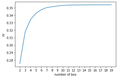
对于特征’age’来说,最佳箱数为6
5. 用最佳分箱数分箱,并验证分箱结果
def get_bin(num_bins_, n):while len(num_bins_) > n:pvs = []for i in range(len(num_bins_) - 1):x1 = num_bins_[i][2:]x2 = num_bins_[i+1][2:]# chi2v = scipy.stats.chi2_contingency([x1, x2])[0] 返回卡方值pv = scipy.stats.chi2_contingency([x1, x2])[1] # 返回p值pvs.append(pv)i = pvs.index(max(pvs))num_bins_[i:i+2] = [(num_bins_[i][0], num_bins_[i+1][1],num_bins_[i][2] + num_bins_[i+1][2],num_bins_[i][3] + num_bins_[i+1][3])]return num_bins_
num_bins_ = num_bins.copy()afterbins = get_bin(num_bins_, 6)afterbins
[(21.0, 36.0, 14797, 24809),(36.0, 54.0, 39070, 51461),(54.0, 61.0, 15743, 12227),(61.0, 64.0, 6968, 3229),(64.0, 74.0, 13376, 4206),(74.0, 107.0, 7737, 1385)]
bins_df = get_woe(afterbins)bins_df
| min | max | count_0 | count_1 | total | percentage | bad_rate | bad% | good% | woe | |
|---|---|---|---|---|---|---|---|---|---|---|
| 0 | 21.0 | 36.0 | 14797 | 24809 | 39606 | 0.203099 | 0.626395 | 0.254930 | 0.151467 | -0.520618 |
| 1 | 36.0 | 54.0 | 39070 | 51461 | 90531 | 0.464242 | 0.568435 | 0.528798 | 0.399934 | -0.279305 |
| 2 | 54.0 | 61.0 | 15743 | 12227 | 27970 | 0.143430 | 0.437147 | 0.125641 | 0.161151 | 0.248913 |
| 3 | 61.0 | 64.0 | 6968 | 3229 | 10197 | 0.052290 | 0.316662 | 0.033180 | 0.071327 | 0.765320 |
| 4 | 64.0 | 74.0 | 13376 | 4206 | 17582 | 0.090160 | 0.239222 | 0.043220 | 0.136922 | 1.153114 |
| 5 | 74.0 | 107.0 | 7737 | 1385 | 9122 | 0.046778 | 0.151831 | 0.014232 | 0.079199 | 1.716478 |
理想情况:每组的bad_rate差异较大,woe趋势单调
包装判断分箱个数的函数
基于卡方检验分箱:
DF:需要输入的特征数据 X:需要分箱的列名 Y:分箱数据对应的标签Y的列名 n:保留箱数 q:初始分箱数 graph:是否画出IV图像 区间为前开后闭 (]
def graphforbestbin(DF, X, Y, n = 5, q = 20, graph = True):DF = DF[[X, Y]].copy()DF['qcut'], updown = pd.qcut(DF[X], retbins = True, q = q, duplicates = 'drop')count_y0 = DF[DF[Y] == 0].groupby(by = 'qcut').count()[Y]count_y1 = DF[DF[Y] == 1].groupby(by = 'qcut').count()[Y]num_bins = [*zip(updown, updown[1:], count_y0, count_y1)]for i in range(q):if 0 in num_bins[0][2:]:num_bins[0:2] = [(num_bins[0][0], num_bins[1][1], num_bins[0][2] + num_bins[1][2], num_bins[0][3] + num_bins[1][3])]continuefor i in range(len(num_bins)):if 0 in num_bins[i][2:]:num_bins[i-1:i+1] = [(num_bins[i-1][0], num_bins[i][1], num_bins[i-1][2] + num_bins[i][2], num_bins[i-1][3] + num_bins[i][3])]breakelse:breakdef get_woe(num_bins):columns = ['min', 'max', 'count_0', 'count_1']df = pd.DataFrame(num_bins, columns = columns)df['total'] = df['count_0'] + df['count_1']df['percentage'] = df['total']/df['total'].sum()df['bad_rate'] = df['count_1']/df['total']df['bad%'] = df['count_1']/df['count_1'].sum()df['good%'] = df['count_0']/df['count_0'].sum()df['woe'] = np.log(df['good%']/df['bad%'])return dfdef get_iv(bins_df):rate = bins_df['good%'] - bins_df['bad%']iv = np.sum(rate * bins_df['woe'])return ivIV = []axisx = []while len(num_bins) > n:pvs = []for i in range(len(num_bins) - 1):x1 = num_bins[i][2:]x2 = num_bins[i+1][2:]pv = scipy.stats.chi2_contingency([x1, x2])[1]pvs.append(pv)i = pvs.index(max(pvs))num_bins[i:i+2] = [(num_bins[i][0], num_bins[i+1][1],num_bins[i][2] + num_bins[i+1][2],num_bins[i][3] + num_bins[i+1][3])]bins_df = pd.DataFrame(get_woe(num_bins))axisx.append(len(num_bins))IV.append(get_iv(bins_df))if graph:plt.figure()plt.plot(axisx, IV)plt.xticks(axisx)plt.xlabel('number of box')plt.ylabel('IV')plt.show()return bins_df
不是所有的特征都可以使用这个分箱函数,如家人数量,就无法分出20组
将可以分箱的特征放出来单独分组,不能自动分箱的变量手动将其分箱
# 可使用函数自动分箱的变量:auto_col_bins = {'RevolvingUtilizationOfUnsecuredLines':6,'age':5,'DebtRatio':4,'MonthlyIncome':3,'NumberOfOpenCreditLinesAndLoans':5}# 不能使用函数自动分箱的变量,手动分箱:hand_bins = {'NumberOfTime30-59DaysPastDueNotWorse':[0, 1, 2, 13],'NumberOfTime60-89DaysPastDueNotWorse':[0, 1, 2, 17],'NumberOfTimes90DaysLate':[0, 1, 2, 4, 54],'NumberRealEstateLoansOrLines':[0, 1, 2, 8],'NumberOfDependents':[0, 1, 2, 3]}# 保证区间覆盖:用负无穷表示最小值,用正无穷表示最大值hand_bins = {k:[-np.inf, *v[:-1], np.inf] for k, v in hand_bins.items()}
hand_bins
{'NumberOfTime30-59DaysPastDueNotWorse': [-inf, 0, 1, 2, inf],'NumberOfTime60-89DaysPastDueNotWorse': [-inf, 0, 1, 2, inf],'NumberOfTimes90DaysLate': [-inf, 0, 1, 2, 4, inf],'NumberRealEstateLoansOrLines': [-inf, 0, 1, 2, inf],'NumberOfDependents': [-inf, 0, 1, 2, inf]}
bins_of_col = {}for col in auto_col_bins:bins_df = graphforbestbin(model_data, col, 'SeriousDlqin2yrs', n = auto_col_bins[col], q = 20, graph = False)# 返回DataFramebins_list = sorted(set(bins_df['min']).union(bins_df['max']))# 返回列表bins_list[0], bins_list[-1] = -np.inf, np.inf# 将列表的最小值和最大值替换为无穷小和无穷大bins_of_col[col] = bins_list# 利用字典的性质,创建键并赋值bins_of_col.update(hand_bins)
bins_df
| min | max | count_0 | count_1 | total | percentage | bad_rate | bad% | good% | woe | |
|---|---|---|---|---|---|---|---|---|---|---|
| 0 | 0.0 | 1.0 | 3393 | 7823 | 11216 | 0.057516 | 0.697486 | 0.080387 | 0.034732 | -0.839189 |
| 1 | 1.0 | 3.0 | 9995 | 13892 | 23887 | 0.122492 | 0.581572 | 0.142750 | 0.102312 | -0.333064 |
| 2 | 3.0 | 5.0 | 16106 | 17014 | 33120 | 0.169839 | 0.513708 | 0.174831 | 0.164867 | -0.058680 |
| 3 | 5.0 | 17.0 | 62732 | 55163 | 117895 | 0.604565 | 0.467899 | 0.566838 | 0.642147 | 0.124744 |
| 4 | 17.0 | 57.0 | 5465 | 3425 | 8890 | 0.045588 | 0.385264 | 0.035194 | 0.055942 | 0.463427 |
bins_list
[-inf, 1.0, 3.0, 5.0, 17.0, inf]
len(bins_of_col)
10
bins_of_col
{'RevolvingUtilizationOfUnsecuredLines': [-inf,0.09901938874999999,0.2977106203246584,0.46504505549999997,0.9823017611053088,0.9999998999999999,inf],'NumberOfTime30-59DaysPastDueNotWorse': [-inf, 0, 1, 2, inf],'NumberOfTime60-89DaysPastDueNotWorse': [-inf, 0, 1, 2, inf],'NumberOfTimes90DaysLate': [-inf, 0, 1, 2, 4, inf],'NumberRealEstateLoansOrLines': [-inf, 0, 1, 2, inf],'NumberOfDependents': [-inf, 0, 1, 2, inf],'age': [-inf, 36.0, 54.0, 61.0, 74.0, inf],'DebtRatio': [-inf,0.017443254267870807,0.3205640818,1.4677944020167184,inf],'MonthlyIncome': [-inf, 0.10442453781397015, 6906.041317550067, inf],'NumberOfOpenCreditLinesAndLoans': [-inf, 1.0, 3.0, 5.0, 17.0, inf]}
映射数据
计算各箱的WOE值,并映射到数据中
data = model_data.copy()data = data[['age', 'SeriousDlqin2yrs']].copy()['cut'] = pd.cut(data['age'], [-np.inf, 36.0, 54.0, 61.0, 74.0, np.inf])
data.groupby('cut').size()
cut(-inf, 36.0] 39606(36.0, 54.0] 90531(54.0, 61.0] 27970(61.0, 74.0] 27779(74.0, inf] 9122dtype: int64
data.groupby('cut')['SeriousDlqin2yrs'].size()
cut(-inf, 36.0] 39606(36.0, 54.0] 90531(54.0, 61.0] 27970(61.0, 74.0] 27779(74.0, inf] 9122Name: SeriousDlqin2yrs, dtype: int64
data.groupby('cut')['SeriousDlqin2yrs'].value_counts()
cut SeriousDlqin2yrs(-inf, 36.0] 1 248090 14797(36.0, 54.0] 1 514610 39070(54.0, 61.0] 0 157431 12227(61.0, 74.0] 0 203441 7435(74.0, inf] 0 77371 1385Name: SeriousDlqin2yrs, dtype: int64
data.groupby('cut')['SeriousDlqin2yrs'].value_counts().unstack()
| SeriousDlqin2yrs | 0 | 1 |
|---|---|---|
| cut | ||
| (-inf, 36.0] | 14797 | 24809 |
| (36.0, 54.0] | 39070 | 51461 |
| (54.0, 61.0] | 15743 | 12227 |
| (61.0, 74.0] | 20344 | 7435 |
| (74.0, inf] | 7737 | 1385 |
bins_df = data.groupby('cut')['SeriousDlqin2yrs'].value_counts().unstack()bins_df['woe'] = np.log((bins_df[0]/bins_df[0].sum())/(bins_df[1]/bins_df[1].sum()))
bins_df
| SeriousDlqin2yrs | 0 | 1 | woe |
|---|---|---|---|
| cut | |||
| (-inf, 36.0] | 14797 | 24809 | -0.520618 |
| (36.0, 54.0] | 39070 | 51461 | -0.279305 |
| (54.0, 61.0] | 15743 | 12227 | 0.248913 |
| (61.0, 74.0] | 20344 | 7435 | 1.002752 |
| (74.0, inf] | 7737 | 1385 | 1.716478 |
def get_woe(df, col, y, bins):df = df[[col, y]].copy()df['cut'] = pd.cut(df[col], bins)bins_df = df.groupby('cut')[y].value_counts().unstack()bins_df['woe'] = np.log((bins_df[0]/bins_df[0].sum())/(bins_df[1]/bins_df[1].sum()))return bins_df['woe']woeall = {}for col in bins_of_col:woeall[col] = get_woe(model_data, col, 'SeriousDlqin2yrs', bins_of_col[col])
model_woe = pd.DataFrame(index = model_data.index)model_woe['age'] = pd.cut(model_data['age'], bins_of_col['age']).map(woeall['age'])
woeall['age']
cut(-inf, 36.0] -0.520618(36.0, 54.0] -0.279305(54.0, 61.0] 0.248913(61.0, 74.0] 1.002752(74.0, inf] 1.716478Name: woe, dtype: float64
model_woe.head()
| age | |
|---|---|
| 0 | -0.279305 |
| 1 | 1.002752 |
| 2 | -0.279305 |
| 3 | 1.002752 |
| 4 | -0.279305 |
for col in bins_of_col:model_woe[col] = pd.cut(model_data[col], bins_of_col[col]).map(woeall[col])model_woe.head()
| age | RevolvingUtilizationOfUnsecuredLines | NumberOfTime30-59DaysPastDueNotWorse | NumberOfTime60-89DaysPastDueNotWorse | NumberOfTimes90DaysLate | NumberRealEstateLoansOrLines | NumberOfDependents | DebtRatio | MonthlyIncome | NumberOfOpenCreditLinesAndLoans | |
|---|---|---|---|---|---|---|---|---|---|---|
| 0 | -0.279305 | 2.200291 | 0.353540 | 0.124668 | 0.234166 | -0.393347 | 0.660019 | 0.072859 | -0.195934 | -0.058680 |
| 1 | 1.002752 | 0.667595 | 0.353540 | 0.124668 | 0.234166 | -0.393347 | 0.660019 | 0.072859 | -0.195934 | -0.058680 |
| 2 | -0.279305 | -2.037728 | -0.873869 | -1.769915 | -1.755182 | -0.393347 | -0.479114 | -0.313585 | -0.195934 | -0.058680 |
| 3 | 1.002752 | 2.200291 | 0.353540 | 0.124668 | 0.234166 | 0.614648 | 0.660019 | -0.313585 | -0.195934 | 0.124744 |
| 4 | -0.279305 | -1.073972 | 0.353540 | 0.124668 | 0.234166 | 0.614648 | -0.512452 | -0.313585 | 0.311098 | 0.124744 |
model_woe['SeriousDlqin2yrs'] = model_data['SeriousDlqin2yrs']
model_woe.head()
| age | RevolvingUtilizationOfUnsecuredLines | NumberOfTime30-59DaysPastDueNotWorse | NumberOfTime60-89DaysPastDueNotWorse | NumberOfTimes90DaysLate | NumberRealEstateLoansOrLines | NumberOfDependents | DebtRatio | MonthlyIncome | NumberOfOpenCreditLinesAndLoans | SeriousDlqin2yrs | |
|---|---|---|---|---|---|---|---|---|---|---|---|
| 0 | -0.279305 | 2.200291 | 0.353540 | 0.124668 | 0.234166 | -0.393347 | 0.660019 | 0.072859 | -0.195934 | -0.058680 | 0 |
| 1 | 1.002752 | 0.667595 | 0.353540 | 0.124668 | 0.234166 | -0.393347 | 0.660019 | 0.072859 | -0.195934 | -0.058680 | 0 |
| 2 | -0.279305 | -2.037728 | -0.873869 | -1.769915 | -1.755182 | -0.393347 | -0.479114 | -0.313585 | -0.195934 | -0.058680 | 1 |
| 3 | 1.002752 | 2.200291 | 0.353540 | 0.124668 | 0.234166 | 0.614648 | 0.660019 | -0.313585 | -0.195934 | 0.124744 | 0 |
| 4 | -0.279305 | -1.073972 | 0.353540 | 0.124668 | 0.234166 | 0.614648 | -0.512452 | -0.313585 | 0.311098 | 0.124744 | 1 |
建模与模型验证
用准确率和ROC曲线验证模型的预测能力和捕捉能力
vali_woe = pd.DataFrame(index = vali_data.index)for col in bins_of_col:vali_woe[col] = pd.cut(vali_data[col], bins_of_col[col]).map(woeall[col])vali_woe['SeriousDlqin2yrs'] = vali_data['SeriousDlqin2yrs']vali_woe.head()
| RevolvingUtilizationOfUnsecuredLines | NumberOfTime30-59DaysPastDueNotWorse | NumberOfTime60-89DaysPastDueNotWorse | NumberOfTimes90DaysLate | NumberRealEstateLoansOrLines | NumberOfDependents | age | DebtRatio | MonthlyIncome | NumberOfOpenCreditLinesAndLoans | SeriousDlqin2yrs | |
|---|---|---|---|---|---|---|---|---|---|---|---|
| 0 | 2.200291 | 0.35354 | 0.124668 | 0.234166 | -0.393347 | 0.660019 | 0.248913 | 1.513332 | -0.195934 | -0.058680 | 0 |
| 1 | -1.073972 | 0.35354 | 0.124668 | 0.234166 | 0.614648 | -0.479114 | -0.279305 | 0.072859 | 0.311098 | 0.124744 | 1 |
| 2 | 2.200291 | 0.35354 | 0.124668 | 0.234166 | -0.393347 | 0.660019 | 1.002752 | 0.072859 | -0.195934 | -0.058680 | 0 |
| 3 | 2.200291 | 0.35354 | 0.124668 | 0.234166 | 0.195778 | 0.660019 | -0.279305 | 0.072859 | -0.195934 | 0.124744 | 0 |
| 4 | -1.073972 | 0.35354 | 0.124668 | 0.234166 | -0.393347 | -0.512452 | -0.279305 | -0.313585 | -0.195934 | 0.124744 | 1 |
vali_x = vali_woe.iloc[:, :-1]vali_y = vali_woe.iloc[:, -1]x = model_woe.iloc[:, :-1]y = model_woe.iloc[:, -1]
lr = LR().fit(x, y)lr.score(x, y)
0.7857421234000657
lr.score(vali_x, vali_y)
0.7651957499760697
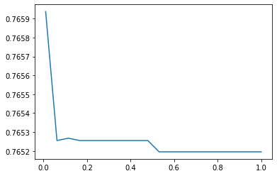
c = np.linspace(0.01, 1, 20)score = []for i in c:lr = LR(solver = 'liblinear', C = i).fit(x, y)score.append(lr.score(vali_x, vali_y))print(lr.n_iter_)plt.figure()plt.plot(c, score)
[5][<matplotlib.lines.Line2D at 0x26224266b00>]
score = []for i in [1, 2, 3, 4, 5, 6]:lr = LR(solver = 'liblinear', C = 0.025, max_iter = i).fit(x, y)score.append(lr.score(vali_x, vali_y))plt.figure()plt.plot([1, 2, 3, 4, 5, 6], score)plt.show()
C:\anaconda\lib\site-packages\sklearn\svm\_base.py:947: ConvergenceWarning: Liblinear failed to converge, increase the number of iterations."the number of iterations.", ConvergenceWarning)C:\anaconda\lib\site-packages\sklearn\svm\_base.py:947: ConvergenceWarning: Liblinear failed to converge, increase the number of iterations."the number of iterations.", ConvergenceWarning)C:\anaconda\lib\site-packages\sklearn\svm\_base.py:947: ConvergenceWarning: Liblinear failed to converge, increase the number of iterations."the number of iterations.", ConvergenceWarning)C:\anaconda\lib\site-packages\sklearn\svm\_base.py:947: ConvergenceWarning: Liblinear failed to converge, increase the number of iterations."the number of iterations.", ConvergenceWarning)C:\anaconda\lib\site-packages\sklearn\svm\_base.py:947: ConvergenceWarning: Liblinear failed to converge, increase the number of iterations."the number of iterations.", ConvergenceWarning)
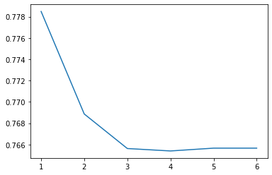
准确率较低。再来看模型在ROC曲线上的结果:
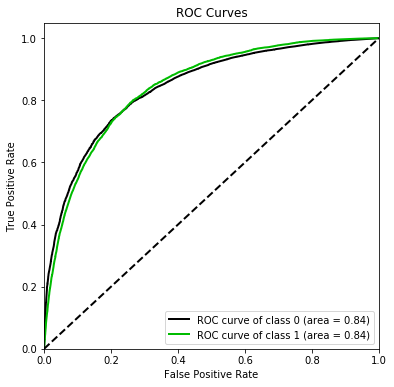
import scikitplot as skpltvali_proba_df = pd.DataFrame(lr.predict_proba(vali_x))skplt.metrics.plot_roc(vali_y, vali_proba_df,plot_micro = False, figsize = (6, 6),plot_macro = False)
<matplotlib.axes._subplots.AxesSubplot at 0x2620dad42b0>
制作评分卡
 其中,A和B是常数,A为“补偿”,B为“刻度”,
 即对数几率,会得到
 ,即参数
,即参数 特征矩阵,代表一个人的违约可能性
两个常数可以通过两个假设的分值代入公式求出:
- 某个特定的违约概率下的预期分值
- 指定的违约概率翻倍的分值(PDO)
例如,假设对数几率为 时,分值为600,PDO为20,即对数几率为
 时的分数为620,代入以上线性表达式可以得到:


求出A和B,分数就很容易得到了。其中不受评分卡各特征影响的基础分,就是将截距作为代入公式计算,而其他各个特征的各个分档的分值,也是将系数代入计算得出:
B = 20/np.log(2)A = 600 + B * np.log(1/60)base_score = A - B * lr.intercept_score_age = woeall['age'] * (-B * lr.coef_[0][1])
base_score
array([481.96632407])
score_age
cut(-inf, 36.0] -11.323029(36.0, 54.0] -6.074667(54.0, 61.0] 5.413673(61.0, 74.0] 21.809064(74.0, inf] 37.332055Name: woe, dtype: float64
file = 'ScoreData.csv'with open(file, 'w') as fdata:fdata.write('base_score, {}\n'.format(base_score))for i, col in enumerate(x.columns):score = woeall[col] * (-B * lr.coef_[0][i])score.name = "Score"score.index.name = colscore.to_csv(file, header = True, mode = 'a')
x.columns
Index(['age', 'RevolvingUtilizationOfUnsecuredLines','NumberOfTime30-59DaysPastDueNotWorse','NumberOfTime60-89DaysPastDueNotWorse', 'NumberOfTimes90DaysLate','NumberRealEstateLoansOrLines', 'NumberOfDependents', 'DebtRatio','MonthlyIncome', 'NumberOfOpenCreditLinesAndLoans'],dtype='object')

若有收获,就点个赞吧
0 人点赞
