一、 数据预处理 preprocessing & impute
1. 数据无量纲化
归一化 Normalization
from sklearn.preprocessing import MinMaxScalerimport numpy as npimport pandas as pd
MinMaxScaler归一化
data = [[-1, 2], [-0.5, 6], [0, 10], [1, 18]]type(data)
list
data
[[-1, 2], [-0.5, 6], [0, 10], [1, 18]]
data = pd.DataFrame(data)type(data)
pandas.core.frame.DataFrame
data
| 0 | 1 | |
|---|---|---|
| 0 | -1.0 | 2 |
| 1 | -0.5 | 6 |
| 2 | 0.0 | 10 |
| 3 | 1.0 | 18 |
norm = MinMaxScaler() # 实例化norm.fit(data) # 生成原始数据的 min 和 maxresult = norm.transform(data) # 通过接口导出结果result
array([[0. , 0. ],[0.25, 0.25],[0.5 , 0.5 ],[1. , 1. ]])
归一化后两列的分布一致,说明两列传递的信息是相近的,甚至是一致的
norm = MinMaxScaler()result_ = norm.fit_transform(data) # 训练和导出结果一步达成result_
array([[0. , 0. ],[0.25, 0.25],[0.5 , 0.5 ],[1. , 1. ]])
norm.inverse_transform(result_) # 逆转归一化的结果
array([[-1. , 2. ],[-0.5, 6. ],[ 0. , 10. ],[ 1. , 18. ]])
scaler = MinMaxScaler(feature_range = [5, 10])scaler.fit_transform(data)
array([[ 5. , 5. ],[ 6.25, 6.25],[ 7.5 , 7.5 ],[10. , 10. ]])
fit 和 partial_fit
当特征数量过多时,fit会报错 此时使用partial_fit作为训练接口 scaler = scaler.partial_fit(data)
numpy归一化
data = [[-1, 2], [-0.5, 6], [0, 10], [1, 18]]x = np.array(data)
x.min()
-1.0
x.min(axis = 0)
array([-1., 2.])
x.min(axis = 1)
array([-1. , -0.5, 0. , 1. ])
x_nor = (x - x.min(axis = 0)) / (x.max(axis = 0) - x.min(axis = 0))x_nor
array([[0. , 0. ],[0.25, 0.25],[0.5 , 0.5 ],[1. , 1. ]])
x_nor * (x.max(axis = 0) - x.min(axis = 0)) + x.min(axis = 0)
array([[-1. , 2. ],[-0.5, 6. ],[ 0. , 10. ],[ 1. , 18. ]])
标准化 Standardization
data = [[-1, 2], [-0.5, 6], [0, 10], [1, 18]]
from sklearn.preprocessing import StandardScalerscaler = StandardScaler()scaler.fit(data) # 生成原始数据的均值和方差
StandardScaler(copy=True, with_mean=True, with_std=True)
scaler.mean_
array([-0.125, 9. ])
scaler.var_
array([ 0.546875, 35. ])
x_std = scaler.transform(data)x_std
array([[-1.18321596, -1.18321596],[-0.50709255, -0.50709255],[ 0.16903085, 0.16903085],[ 1.52127766, 1.52127766]])
x_std.mean()
0.0
x_std.var()
1.0
x_std.std()
1.0
scaler.inverse_transform(x_std)
array([[-1. , 2. ],[-0.5, 6. ],[ 0. , 10. ],[ 1. , 18. ]])
无量纲化算法选择
- 大多数机器学习算法中,会选择StandardScaler进行特征缩放,而MinMaxScaler对异常值过于敏感
- MinMaxScaler在不涉及距离度量,梯度,协方差以及数据需要被压缩到特定区间的时候,应用广泛
- 在压缩数据却不希望影响数据的稀疏性(不影响矩阵中取值为0的个数)时,只缩放不进行中心化,选用MaxAbsScaler
- 在异常值多,噪声非常大的时候,选择分位数来无量纲化,选用RobustScaler
稀疏数据
在数据库中,稀疏数据是指在二维表中含有大量空值的数据;
即稀疏数据是指,在数据集中绝大多数数值缺失或者为零的数据。
稀疏数据绝对不是无用数据,只不过是信息不完全,通过适当的手段是可以挖掘出大量有用信息。
2. 缺失值处理
data = pd.read_csv('Narrativedata.csv', index_col = 0)
data.head()
| Age | Sex | Embarked | Survived | |
|---|---|---|---|---|
| 0 | 22.0 | male | S | No |
| 1 | 38.0 | female | C | Yes |
| 2 | 26.0 | female | S | Yes |
| 3 | 35.0 | female | S | Yes |
| 4 | 35.0 | male | S | No |
data.info()
<class 'pandas.core.frame.DataFrame'>Int64Index: 891 entries, 0 to 890Data columns (total 4 columns):Age 714 non-null float64Sex 891 non-null objectEmbarked 889 non-null objectSurvived 891 non-null objectdtypes: float64(1), object(3)memory usage: 34.8+ KB
Age = data.loc[:, 'Age'].values.reshape(-1, 1)# data.loc[:, 'Age'] 提取出Series,由一列数据和对应的索引组成# data.loc[:, 'Age'].values 将Series转换为array,才可以使用array的方法reshape将年龄数据从一维转为二维
from sklearn.impute import SimpleImputerimp_mean = SimpleImputer()imp_median = SimpleImputer(strategy = 'median')imp_zero = SimpleImputer(strategy = 'constant', fill_value = 0)imp_mean = imp_mean.fit_transform(Age)imp_median = imp_median.fit_transform(Age)imp_zero = imp_zero.fit_transform(Age)
imp_mean[:10]
array([[22. ],[38. ],[26. ],[35. ],[35. ],[29.69911765],[54. ],[ 2. ],[27. ],[14. ]])
imp_median[:10]
array([[22.],[38.],[26.],[35.],[35.],[28.],[54.],[ 2.],[27.],[14.]])
imp_zero[:10]
array([[22.],[38.],[26.],[35.],[35.],[ 0.],[54.],[ 2.],[27.],[14.]])
data['Age'] = imp_median# 年龄通常用均值填补,但在这里中位数和均值相差不大,且中位数为整数,所以选择中位数来填补
data.info()
<class 'pandas.core.frame.DataFrame'>Int64Index: 891 entries, 0 to 890Data columns (total 4 columns):Age 891 non-null float64Sex 891 non-null objectEmbarked 889 non-null objectSurvived 891 non-null objectdtypes: float64(1), object(3)memory usage: 34.8+ KB
Embarked = data['Embarked'].values.reshape(-1, 1)
imp_mode = SimpleImputer(strategy = 'most_frequent')imp_mode = imp_mode.fit_transform(Embarked)
data.Embarked = imp_mode
data.info()
<class 'pandas.core.frame.DataFrame'>Int64Index: 891 entries, 0 to 890Data columns (total 4 columns):Age 891 non-null float64Sex 891 non-null objectEmbarked 891 non-null objectSurvived 891 non-null objectdtypes: float64(1), object(3)memory usage: 34.8+ KB
用pandas和numpy填补更方便
data_ = pd.read_csv('Narrativedata.csv', index_col = 0)data_.head()
| Age | Sex | Embarked | Survived | |
|---|---|---|---|---|
| 0 | 22.0 | male | S | No |
| 1 | 38.0 | female | C | Yes |
| 2 | 26.0 | female | S | Yes |
| 3 | 35.0 | female | S | Yes |
| 4 | 35.0 | male | S | No |
data_.info()
<class 'pandas.core.frame.DataFrame'>Int64Index: 891 entries, 0 to 890Data columns (total 4 columns):Age 714 non-null float64Sex 891 non-null objectEmbarked 889 non-null objectSurvived 891 non-null objectdtypes: float64(1), object(3)memory usage: 34.8+ KB
data_.Age = data_.Age.fillna(data_.Age.median())
data_.info()
<class 'pandas.core.frame.DataFrame'>Int64Index: 891 entries, 0 to 890Data columns (total 4 columns):Age 891 non-null float64Sex 891 non-null objectEmbarked 889 non-null objectSurvived 891 non-null objectdtypes: float64(1), object(3)memory usage: 34.8+ KB
data_.dropna(axis = 0, inplace = True)
data_.info()
<class 'pandas.core.frame.DataFrame'>Int64Index: 889 entries, 0 to 890Data columns (total 4 columns):Age 889 non-null float64Sex 889 non-null objectEmbarked 889 non-null objectSurvived 889 non-null objectdtypes: float64(1), object(3)memory usage: 34.7+ KB
3. 处理分类型特征和标签
LabelEncoder
from sklearn.preprocessing import LabelEncoder
y = data.iloc[:, -1]le = LabelEncoder() # 实例化le.fit(y) # 导入数据y = le.transform(y) # transform接口调取数据y[:5]
array([0, 2, 2, 2, 0])
le.classes_ # 查看类别
array(['No', 'Unknown', 'Yes'], dtype=object)
data.iloc[:, -1] = ydata.head()
| Age | Sex | Embarked | Survived | |
|---|---|---|---|---|
| 0 | 22.0 | male | S | 0 |
| 1 | 38.0 | female | C | 2 |
| 2 | 26.0 | female | S | 2 |
| 3 | 35.0 | female | S | 2 |
| 4 | 35.0 | male | S | 0 |
# 简化写法from sklearn.preprocessing import LabelEncoderdata.iloc[:, -1] = LabelEncoder().fit_transform(data.iloc[:, -1])
OrdinalEncoder
from sklearn.preprocessing import OrdinalEncoder
data_ = data.copy()data_.head()
| Age | Sex | Embarked | Survived | |
|---|---|---|---|---|
| 0 | 22.0 | male | S | 0 |
| 1 | 38.0 | female | C | 2 |
| 2 | 26.0 | female | S | 2 |
| 3 | 35.0 | female | S | 2 |
| 4 | 35.0 | male | S | 0 |
OrdinalEncoder().fit(data_.iloc[:, 1:-1]).categories_
[array(['female', 'male'], dtype=object), array(['C', 'Q', 'S'], dtype=object)]
data_.iloc[:, 1:-1] = OrdinalEncoder().fit_transform(data_.iloc[:, 1:-1])
OrdinalEncoder().fit(data_.iloc[:, 1:-1]).categories_
[array([0., 1.]), array([0., 1., 2.])]
data_.head()
| Age | Sex | Embarked | Survived | |
|---|---|---|---|---|
| 0 | 22.0 | 1.0 | 2.0 | 0 |
| 1 | 38.0 | 0.0 | 0.0 | 2 |
| 2 | 26.0 | 0.0 | 2.0 | 2 |
| 3 | 35.0 | 0.0 | 2.0 | 2 |
| 4 | 35.0 | 1.0 | 2.0 | 0 |
OneHotEncoder
from sklearn.preprocessing import OneHotEncoderresult = OneHotEncoder(categories = 'auto').fit_transform(data.iloc[:, 1:-1]).toarray()result
array([[0., 1., 0., 0., 1.],[1., 0., 1., 0., 0.],[1., 0., 0., 0., 1.],...,[1., 0., 0., 0., 1.],[0., 1., 1., 0., 0.],[0., 1., 0., 1., 0.]])
OneHotEncoder(categories = 'auto').fit(data.iloc[:, 1:-1]).get_feature_names()
array(['x0_female', 'x0_male', 'x1_C', 'x1_Q', 'x1_S'], dtype=object)
result.shape
(891, 5)
newdata = pd.concat([data, pd.DataFrame(result)], axis = 1)newdata.head()
| Age | Sex | Embarked | Survived | 0 | 1 | 2 | 3 | 4 | |
|---|---|---|---|---|---|---|---|---|---|
| 0 | 22.0 | male | S | 0 | 0.0 | 1.0 | 0.0 | 0.0 | 1.0 |
| 1 | 38.0 | female | C | 2 | 1.0 | 0.0 | 1.0 | 0.0 | 0.0 |
| 2 | 26.0 | female | S | 2 | 1.0 | 0.0 | 0.0 | 0.0 | 1.0 |
| 3 | 35.0 | female | S | 2 | 1.0 | 0.0 | 0.0 | 0.0 | 1.0 |
| 4 | 35.0 | male | S | 0 | 0.0 | 1.0 | 0.0 | 0.0 | 1.0 |
newdata.iloc[:, -5:].columns
Index([0, 1, 2, 3, 4], dtype='object')
newdata.drop(['Age', 'Embarked'], axis = 1, inplace = True)newdata.columns = ['Age', 'Survived', 'female', 'male', 'C', 'Q', 'S']newdata.head()
| Age | Survived | female | male | C | Q | S | |
|---|---|---|---|---|---|---|---|
| 0 | male | 0 | 0.0 | 1.0 | 0.0 | 0.0 | 1.0 |
| 1 | female | 2 | 1.0 | 0.0 | 1.0 | 0.0 | 0.0 |
| 2 | female | 2 | 1.0 | 0.0 | 0.0 | 0.0 | 1.0 |
| 3 | female | 2 | 1.0 | 0.0 | 0.0 | 0.0 | 1.0 |
| 4 | male | 0 | 0.0 | 1.0 | 0.0 | 0.0 | 1.0 |
4. 处理连续型特征
在统计和机器学习中,离散化是指将连续属性,特征或变量转换或划分为离散或标称属性/特征/变量/间隔的过程。
它是一种离散化的形式,也可以是分组,如制作直方图。每当连续数据离散化时,总会存在一定程度的离散化误差。
离散化的目标是将数量减少到建模可忽略不计的水平。
二值化 Binarizer
from sklearn.preprocessing import Binarizerdata_2 = data.copy()X = data_2.iloc[:, 0].values.reshape(-1, 1)transformer = Binarizer(threshold = 30).fit_transform(X)
transformer[:10]
array([[0.],[1.],[0.],[1.],[1.],[0.],[1.],[0.],[0.],[0.]])
data_2.iloc[:, 0] = transformer
data_2.head()
| Age | Sex | Embarked | Survived | |
|---|---|---|---|---|
| 0 | 0.0 | male | S | 0 |
| 1 | 1.0 | female | C | 2 |
| 2 | 0.0 | female | S | 2 |
| 3 | 1.0 | female | S | 2 |
| 4 | 1.0 | male | S | 0 |
y = data_2.iloc[:, -1].values.reshape(-1, 1)transformer = Binarizer(threshold = 1).fit_transform(y)
data_2.iloc[:, -1] = transformer
data_2.head()
| Age | Sex | Embarked | Survived | |
|---|---|---|---|---|
| 0 | 0.0 | male | S | 0 |
| 1 | 1.0 | female | C | 1 |
| 2 | 0.0 | female | S | 1 |
| 3 | 1.0 | female | S | 1 |
| 4 | 1.0 | male | S | 0 |
分箱 KBinsDiscretizer
from sklearn.preprocessing import KBinsDiscretizerX = data.iloc[:, 0].values.reshape(-1, 1)X_tran = KBinsDiscretizer(n_bins = 3, encode = 'ordinal', strategy = 'uniform').fit_transform(X)
data_3 = pd.DataFrame()data_3 = pd.concat([data, pd.DataFrame(X_tran)], axis = 1)
data_3.head()
| Age | Sex | Embarked | Survived | 0 | |
|---|---|---|---|---|---|
| 0 | 22.0 | male | S | 0 | 0.0 |
| 1 | 38.0 | female | C | 2 | 1.0 |
| 2 | 26.0 | female | S | 2 | 0.0 |
| 3 | 35.0 | female | S | 2 | 1.0 |
| 4 | 35.0 | male | S | 0 | 1.0 |
dim_reduce = X_tran.ravel()set(dim_reduce)
{0.0, 1.0, 2.0}
X_tran = KBinsDiscretizer(n_bins = 3, encode = 'onehot', strategy = 'uniform').fit_transform(X)
X_tran
<891x3 sparse matrix of type '<class 'numpy.float64'>'with 891 stored elements in Compressed Sparse Row format>
X_tran.toarray()
array([[1., 0., 0.],[0., 1., 0.],[1., 0., 0.],...,[0., 1., 0.],[1., 0., 0.],[0., 1., 0.]])
二、 特征选择 feature_selection
import pandas as pddata = pd.read_csv("digit recognizor.csv")
C:\anaconda\lib\importlib\_bootstrap.py:219: RuntimeWarning: numpy.ufunc size changed, may indicate binary incompatibility. Expected 192 from C header, got 216 from PyObjectreturn f(*args, **kwds)C:\anaconda\lib\importlib\_bootstrap.py:219: RuntimeWarning: numpy.ufunc size changed, may indicate binary incompatibility. Expected 192 from C header, got 216 from PyObjectreturn f(*args, **kwds)
data.head()
| label | pixel0 | pixel1 | pixel2 | pixel3 | pixel4 | pixel5 | pixel6 | pixel7 | pixel8 | … | pixel774 | pixel775 | pixel776 | pixel777 | pixel778 | pixel779 | pixel780 | pixel781 | pixel782 | pixel783 | |
|---|---|---|---|---|---|---|---|---|---|---|---|---|---|---|---|---|---|---|---|---|---|
| 0 | 1 | 0 | 0 | 0 | 0 | 0 | 0 | 0 | 0 | 0 | … | 0 | 0 | 0 | 0 | 0 | 0 | 0 | 0 | 0 | 0 |
| 1 | 0 | 0 | 0 | 0 | 0 | 0 | 0 | 0 | 0 | 0 | … | 0 | 0 | 0 | 0 | 0 | 0 | 0 | 0 | 0 | 0 |
| 2 | 1 | 0 | 0 | 0 | 0 | 0 | 0 | 0 | 0 | 0 | … | 0 | 0 | 0 | 0 | 0 | 0 | 0 | 0 | 0 | 0 |
| 3 | 4 | 0 | 0 | 0 | 0 | 0 | 0 | 0 | 0 | 0 | … | 0 | 0 | 0 | 0 | 0 | 0 | 0 | 0 | 0 | 0 |
| 4 | 0 | 0 | 0 | 0 | 0 | 0 | 0 | 0 | 0 | 0 | … | 0 | 0 | 0 | 0 | 0 | 0 | 0 | 0 | 0 | 0 |
5 rows × 785 columns
x = data.iloc[:, 1:]y = data.iloc[:, 0]
x.shape
(42000, 784)
数据量大,大在维度高,而非记录多,若不经处理直接带入模型,费时费力
以这个数据集为例,更能看出特征工程的重要性
y.shape
(42000,)
1. Filter过滤法
方差过滤 Variance Threshold
from sklearn.feature_selection import VarianceThreshold
x_var0 = VarianceThreshold().fit_transform(x)
x_var0.shape
(42000, 708)
过滤掉了76个方差为0的特征
x.var().values[:10]
array([0., 0., 0., 0., 0., 0., 0., 0., 0., 0.])
np.median(x.var())
1352.286703180131
x_var_half = VarianceThreshold(np.median(x.var())).fit_transform(x)
x_var_half.shape
(42000, 392)
过滤掉了392个方差小于原始数据的方差中位数的特征
np.array([0, 1, 0, 1, 0, 0, 0, 1, 0, 1]).var()
0.24
当特征为二分类时,特征的取值就是伯努利随机变量(0, 1)
伯努利变量的方差计算公式为:$Var(X) = p * (1-p)$
其中X为二分类特征矩阵,p是二分类特征中某一类所占的概率
# 若特征是伯努利随机变量,当p=0.8,即二分类特征中某种分类占到80%,此时方差为0.8*(1-0.8)=0.16# 令threshold=0.16,即删除有一分类占到80%以上的二分类特征x_bvar = VarianceThreshold(0.16).fit_transform(x)
x_bvar.shape
(42000, 685)
过滤掉了99个二分类特征
方差过滤特征是否提升了模型的效果?
- 模型运行的判别效果(准确率)
- 运行时间
对比KNN和随机森林在中位数方差过滤下的效果
KNN 方差过滤前,模型交叉验证效果:0.9658569700000001 方差过滤后,模型交叉验证效果:0.9659997459999999
随机森林 方差过滤前,模型交叉验证效果:0.9380003861799541 方差过滤后,模型交叉验证效果:0.9388098166696807
# 导入模块并准备数据from sklearn.ensemble import RandomForestClassifier as RFCfrom sklearn.neighbors import KNeighborsClassifier as KNNfrom sklearn.model_selection import cross_val_scorex = data.iloc[:, 1:]y = data.iloc[:, 0]x_var_half = VarianceThreshold(np.median(x.var())).fit_transform(x)
cross_val_score(KNN(), x, y, cv = 5)
array([0.96799524, 0.96548852, 0.96356709, 0.96332023, 0.96891377])
np.array([0.96799524, 0.96548852, 0.96356709, 0.96332023, 0.96891377]).mean()
0.9658569700000001
cross_val_score(KNN(), x_var_half, y, cv = 5)
array([0.96799524, 0.96632155, 0.96368615, 0.96332023, 0.96867556])
np.array([0.96799524, 0.96632155, 0.96368615, 0.96332023, 0.96867556]).mean()
0.9659997459999999
rfc_score1 = cross_val_score(RFC(n_estimators = 10, random_state = 0), x, y, cv = 5)rfc_score1.mean()
0.9380003861799541
%%timeitrfc_score1 = cross_val_score(RFC(n_estimators = 10, random_state = 0), x, y, cv = 5)
13.6 s ± 1.1 s per loop (mean ± std. dev. of 7 runs, 1 loop each)
rfc_score2 = cross_val_score(RFC(n_estimators = 10, random_state = 0), x_var_half, y, cv = 5)rfc_score2.mean()
0.9388098166696807
%%timeitrfc_score2 = cross_val_score(RFC(n_estimators = 10, random_state = 0), x_var_half, y, cv = 5)
12.5 s ± 319 ms per loop (mean ± std. dev. of 7 runs, 1 loop each)
threshold
在机器学习的上下文中,超参数是在开始学习过程之前设置值的参数,而不是通过训练得到的参数数据。 通常情况下,需要对超参数进行优化,给学习机选择一组最优超参数,以提高学习的性能和效果。
相关性过滤
卡方过滤,针对离散型标签(分类问题)
feature_selection.chi2 计算每个非负特征和标签之间的卡方统计量 feature_selection.SelectKBest 按输入的评分标准选出前K个分数最高的特征
from sklearn.feature_selection import chi2from sklearn.feature_selection import SelectKBest
k = SelectKBest(chi2, k = 300).fit_transform(x_var_half, y)k.shape
(42000, 300)
cross_val_score(RFC(n_estimators = 10, random_state = 0), k, y, cv = 5).mean()
0.9333098667649198
在392个特征中保留300个特征,准确率下降
from matplotlib import pyplot as plt%matplotlib inline
score = []for i in range(390, 200, -10):k = SelectKBest(chi2, i).fit_transform(x_var_half, y)once = cross_val_score(RFC(n_estimators = 10, random_state = 0), k, y, cv = 5).mean()score.append(once)plt.plot(range(390, 200, -10), score)
[<matplotlib.lines.Line2D at 0x2461e846a90>]
chivalue, pvalue_chi = chi2(x_var_half, y)
chivalue[:10]
array([ 945664.84392643, 1244766.05139164, 1554872.30384525,1834161.78305343, 1903618.94085294, 1845226.62427198,1602117.23307537, 708535.17489837, 974050.20513718,1188092.19961931])
np.unique(pvalue_chi)
array([0.])
所有特征的p值都小于0.05,说明所有的特征都和标签相关
k = chivalue.shape[0] - (pvalue_chi > 0.05).sum()k
392
F检验
ANOVA,方差齐性检验,用来捕捉每个特征与标签之间的线性关系
feature_selection.f_classif feature_selection.f_regression
from sklearn.feature_selection import f_classifF, pvalue_f = f_classif(x_var_half, y)k = F.shape[0] - (pvalue_f > 0.05).sum()
k
392
互信息法
互信息法用来捕捉每个特征和标签之间的任意关系,包括 线性 和 非线性 关系
feature_selection.mutual_info_classif feature_selection.mutual_info_regression
from sklearn.feature_selection import mutual_info_classif
result = mutual_info_classif(x_var_half, y)k = result.shape[0] - (result <= 0).sum()
k
392
2. Embedded嵌入法
feature_selection.SelectFromModel
from sklearn.feature_selection import SelectFromModel
# 随机森林的实例化RFC_ = RFC(n_estimators = 10, random_state = 0)# SelectFromModel的实例化:SelectFromModel(RFC_, threshold = 0.005)X_embedded = SelectFromModel(RFC_, threshold = 0.005).fit_transform(x, y)
X_embedded.shape
(42000, 47)
importances = RFC_.fit(x, y).feature_importances_importances.max()
0.01276360214820271
threshold = np.linspace(0, importances.max(), 20)threshold
array([0. , 0.00067177, 0.00134354, 0.00201531, 0.00268707,0.00335884, 0.00403061, 0.00470238, 0.00537415, 0.00604592,0.00671769, 0.00738945, 0.00806122, 0.00873299, 0.00940476,0.01007653, 0.0107483 , 0.01142007, 0.01209183, 0.0127636 ])
score = []for i in threshold:X_embedded = SelectFromModel(RFC_, threshold = i).fit_transform(x, y)once = cross_val_score(RFC_, X_embedded, y, cv = 5).mean()score.append(once)plt.plot(threshold, score)
[<matplotlib.lines.Line2D at 0x24620a068d0>]
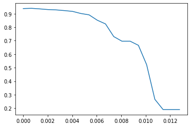
[*zip(threshold, score)]
[(0.0, 0.9380003861799541),(0.000671768534115932, 0.939905083368037),(0.001343537068231864, 0.9356900373288164),(0.002015305602347796, 0.9306673521719839),(0.002687074136463728, 0.9282624651248446),(0.0033588426705796603, 0.923095721100568),(0.004030611204695592, 0.9170958532189901),(0.0047023797388115246, 0.9015485971667836),(0.005374148272927456, 0.8915237372973654),(0.006045916807043388, 0.8517627553998419),(0.0067176853411593206, 0.8243101686902852),(0.007389453875275252, 0.7305249229105348),(0.008061222409391184, 0.6961659491147189),(0.008732990943507116, 0.6961659491147189),(0.009404759477623049, 0.6656903457724771),(0.01007652801173898, 0.5222374843202717),(0.010748296545854913, 0.2654045352411921),(0.011420065079970844, 0.18971438901493287),(0.012091833614086776, 0.18971438901493287),(0.01276360214820271, 0.18971438901493287)]
X_embedded = SelectFromModel(RFC_, threshold = 0.000671768534115932).fit_transform(x, y)X_embedded.shape
(42000, 324)
cross_val_score(RFC_, X_embedded, y, cv = 5).mean()
0.939905083368037
score2 = []for i in np.linspace(0, 0.00134, 20):X_embedded = SelectFromModel(RFC_, threshold = i).fit_transform(x, y)once = cross_val_score(RFC_, X_embedded, y, cv = 5).mean()score2.append(once)plt.figure(figsize = (20, 5))plt.plot(np.linspace(0, 0.00134, 20), score2)plt.xticks(np.linspace(0, 0.00134, 20))
([<matplotlib.axis.XTick at 0x2462083bdd8>,<matplotlib.axis.XTick at 0x2462083fcf8>,<matplotlib.axis.XTick at 0x2462083f668>,<matplotlib.axis.XTick at 0x24ad01a37f0>,<matplotlib.axis.XTick at 0x24ad01a3cc0>,<matplotlib.axis.XTick at 0x24ad01a91d0>,<matplotlib.axis.XTick at 0x24ad01a96a0>,<matplotlib.axis.XTick at 0x24ad01a9b70>,<matplotlib.axis.XTick at 0x24ad01ad0f0>,<matplotlib.axis.XTick at 0x24ad01ad550>,<matplotlib.axis.XTick at 0x24ad01ada20>,<matplotlib.axis.XTick at 0x24ad01adef0>,<matplotlib.axis.XTick at 0x24ad01ad898>,<matplotlib.axis.XTick at 0x24ad01a9b38>,<matplotlib.axis.XTick at 0x24ad01a3898>,<matplotlib.axis.XTick at 0x24ad01b26a0>,<matplotlib.axis.XTick at 0x24ad01b2b70>,<matplotlib.axis.XTick at 0x24ad01b60f0>,<matplotlib.axis.XTick at 0x24ad01b6550>,<matplotlib.axis.XTick at 0x24ad01b6a20>],<a list of 20 Text xticklabel objects>)
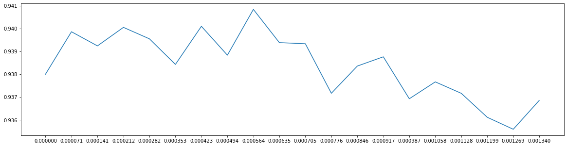
X_embedded = SelectFromModel(RFC_, threshold = 0.000564).fit_transform(x, y)cross_val_score(RFC_, X_embedded, y, cv = 5).mean()
0.9408335415056387
X_embedded.shape
(42000, 340)
X_embedded = SelectFromModel(RFC_, threshold = 0.000564).fit_transform(x, y)cross_val_score(RFC(n_estimators = 100, random_state = 0), X_embedded, y, cv = 5).mean()
0.9639525817795566
3. Wrapper包装法
feature_selection.RFE feature_selection.RFECV
from sklearn.feature_selection import RFEfrom sklearn.ensemble import RandomForestClassifier as RFCfrom sklearn.model_selection import cross_val_scoreimport matplotlib.pyplot as plt%matplotlib inline
RFC_ = RFC(n_estimators = 10, random_state = 0)selector = RFE(RFC_, n_features_to_select = 340, step = 50).fit(x, y)
selector.support_.sum()
340
selector.ranking_[:10]
array([10, 9, 8, 7, 6, 6, 6, 6, 6, 6])
X_wrapper = selector.transform(x)
cross_val_score(RFC_, X_wrapper, y, cv = 5).mean()
0.9389522459432109
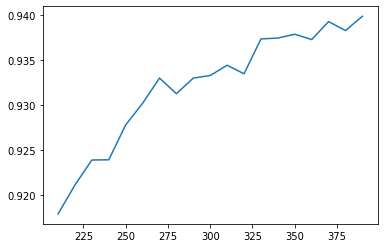
# 画出包装法的学习曲线score = []for i in range(1, 751, 50):X_wrapper = RFE(RFC_, n_features_to_select = i, step = 50).fit_transform(x, y)once = cross_val_score(RFC_, X_wrapper, y, cv = 5).mean()score.append(once)plt.figure(figsize = [20, 5])plt.plot(range(1, 751, 50), score)plt.xticks(range(1, 751, 50))
([<matplotlib.axis.XTick at 0x17a2a8b5898>,<matplotlib.axis.XTick at 0x17a2a8cd128>,<matplotlib.axis.XTick at 0x17a2a8cd320>,<matplotlib.axis.XTick at 0x17a0e0ce6d8>,<matplotlib.axis.XTick at 0x17a0e0ceb70>,<matplotlib.axis.XTick at 0x17a0e0cee80>,<matplotlib.axis.XTick at 0x17a0e0d9550>,<matplotlib.axis.XTick at 0x17a0e0d9ac8>,<matplotlib.axis.XTick at 0x17a0e0dc0f0>,<matplotlib.axis.XTick at 0x17a0e0dc5f8>,<matplotlib.axis.XTick at 0x17a0e0dcb70>,<matplotlib.axis.XTick at 0x17a0e0e0160>,<matplotlib.axis.XTick at 0x17a0e0e06a0>,<matplotlib.axis.XTick at 0x17a0e0dc9e8>,<matplotlib.axis.XTick at 0x17a0e0cef60>],<a list of 15 Text xticklabel objects>)
[*zip(range(1, 751, 50), score)]
[(1, 0.21014266614748944),(51, 0.9085484398226157),(101, 0.924928711799029),(151, 0.9310242511366686),(201, 0.9363097850232442),(251, 0.9353575512540064),(301, 0.9384290399778331),(351, 0.938905032072306),(401, 0.9372626252970612),(451, 0.9398097941390517),(501, 0.9387144536851132),(551, 0.9395716620079153),(601, 0.9385243603795994),(651, 0.9380951142673439),(701, 0.937214229660641)]
三、 特征创造:sklearn中的降维算法

1. 高维数据可视化
from sklearn.datasets import load_irisfrom sklearn.decomposition import PCA
iris = load_iris() # 数据集实例化x = iris.datay = iris.targetx.shape
(150, 4)
二维数组,四维特征
pca = PCA(n_components = 2) # 实例化pca = pca.fit(x) # 拟合模型x_dr = pca.transform(x) # 获取新矩阵
x_dr.shape
(150, 2)
plt.figure(figsize = (10, 6))for i in [0, 1, 2]:plt.scatter(x_dr[y == i, 0], x_dr[y == i, 1],label = iris.target_names[i])plt.legend()plt.title('PCA of IRIS dataset')
Text(0.5, 1.0, 'PCA of IRIS dataset')
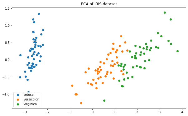
这种分布,距离类模型非常擅长
2. n_components
参照累积可解释方差贡献率曲线 最大似然估计自选 按信息量占比选
累积可解释方差贡献率曲线
pca.explained_variance_# 查看降维后每个新特征向量上所带的信息量的大小# 即可解释性方差的大小
array([4.22824171, 0.24267075])
pca.explained_variance_ratio_# 查看降维后每个新特征向量所占的信息量,占原始数据总信息量的百分比# 又称可解释性方差贡献率
array([0.92461872, 0.05306648])
大部分信息都被集中在第一个特征上
pca.explained_variance_ratio_.sum()
0.9776852063187949
pca_line = PCA().fit(x)pca_line.explained_variance_ratio_.sum()
1.0
import numpy as np
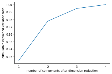
np.cumsum(pca_line.explained_variance_ratio_)
array([0.92461872, 0.97768521, 0.99478782, 1. ])
plt_line = PCA().fit(x)plt.plot([1, 2, 3, 4], # 避免x为y的索引 [0, 1, 2, 3]np.cumsum(pca_line.explained_variance_ratio_))plt.xticks([1, 2, 3, 4]) # 让坐标轴刻度显示为整数plt.xlabel('number of components after dimension reduction')plt.ylabel('cumulative explained variance ratio')
Text(0, 0.5, 'cumulative explained variance ratio')
最大似然估计自选超参数
pca_f = PCA(n_components = 'mle')pca_f = pca_f.fit(x)pca_f.explained_variance_ratio_.sum()
0.9947878161267246
pca_f.explained_variance_ratio_
array([0.92461872, 0.05306648, 0.01710261])
按信息量占比选
前提是,我们知道模型正常运行所需的最少信息量
pca_f = PCA(n_components = 0.99)pca_f = pca_f.fit(x)pca_f.explained_variance_ratio_.sum()
0.9947878161267246
pca_f.explained_variance_ratio_
array([0.92461872, 0.05306648, 0.01710261])
pca_f = PCA(n_components = 0.99, svd_solver = 'full')pca_f = pca_f.fit(x)pca_f.explained_variance_ratio_.sum()
0.9947878161267246
pca_f.explained_variance_ratio_
array([0.92461872, 0.05306648, 0.01710261])
3. svd_solver 奇异值分解器
获得特征空间V(k, n),保存在属性components_中
pca_f = PCA(n_components = k, svd_solver = ‘full’) pca_f = pca_f.fit(x)
将x映射到特征空间V(k, n)上,生成降维后的特征矩阵
x_f = pca_f.transform(x)
PCA(n_components = 2, svd_solver = 'full').fit(x).components_
array([[ 0.36138659, -0.08452251, 0.85667061, 0.3582892 ],[ 0.65658877, 0.73016143, -0.17337266, -0.07548102]])
PCA(2).fit(x).components_
array([[ 0.36138659, -0.08452251, 0.85667061, 0.3582892 ],[ 0.65658877, 0.73016143, -0.17337266, -0.07548102]])
svd_slover默认为auto
4. components_
PCA与特征选择的区别:
特征选择后的特征矩阵可以解读 PCA是压缩已存在的特征,降维后的特征不是原本特征矩阵中的任一特征,不可读
【注意】PCA的目标:在原有特征上找出让信息尽可能聚集的新特征向量
在sklearn使用的PCA和SVD联合的降维算法中,这些新特征向量组成的新特征空间就是V(k, n)
当V(k, n)是数字时,无法判断V(k, n)和原有的特征间的关系 当原特征矩阵是图像,且V(k, n)可视化,通过两张图的对比,可以看出新特征空间如何从原始数据提取信息
from sklearn.datasets import fetch_lfw_peoplefrom sklearn.decomposition import PCA
faces = fetch_lfw_people(min_faces_per_person = 60)
faces.data.shape
(964, 2914)
faces.images.shape
(964, 62, 47)
fig, ax = plt.subplots(4, 5, figsize = [8, 4])
fig, axes = plt.subplots(4, 5, figsize = [8, 4],subplot_kw = {'xticks':[], 'yticks':[]} # 不显示坐标轴)

fig

axes
array([[<matplotlib.axes._subplots.AxesSubplot object at 0x0000017A0F540F28>,<matplotlib.axes._subplots.AxesSubplot object at 0x0000017A0F7F9DD8>,<matplotlib.axes._subplots.AxesSubplot object at 0x0000017A0F7AB4E0>,<matplotlib.axes._subplots.AxesSubplot object at 0x0000017A11CD4EF0>,<matplotlib.axes._subplots.AxesSubplot object at 0x0000017A11D114E0>],[<matplotlib.axes._subplots.AxesSubplot object at 0x0000017A11D40A90>,<matplotlib.axes._subplots.AxesSubplot object at 0x0000017A11D80080>,<matplotlib.axes._subplots.AxesSubplot object at 0x0000017A11DAE5F8>,<matplotlib.axes._subplots.AxesSubplot object at 0x0000017A11DDFBE0>,<matplotlib.axes._subplots.AxesSubplot object at 0x0000017A11E1F1D0>],[<matplotlib.axes._subplots.AxesSubplot object at 0x0000017A11E4D780>,<matplotlib.axes._subplots.AxesSubplot object at 0x0000017A11E7CD30>,<matplotlib.axes._subplots.AxesSubplot object at 0x0000017A11EB9320>,<matplotlib.axes._subplots.AxesSubplot object at 0x0000017A11EEA8D0>,<matplotlib.axes._subplots.AxesSubplot object at 0x0000017A11F1CE80>],[<matplotlib.axes._subplots.AxesSubplot object at 0x0000017A11F58470>,<matplotlib.axes._subplots.AxesSubplot object at 0x0000017A11F89A20>,<matplotlib.axes._subplots.AxesSubplot object at 0x0000017A11FBCFD0>,<matplotlib.axes._subplots.AxesSubplot object at 0x0000017A11FF85C0>,<matplotlib.axes._subplots.AxesSubplot object at 0x0000017A12029B70>]],dtype=object)
axes.shape
(4, 5)
axes[0][0].imshow(faces.images[0, :, :])
<matplotlib.image.AxesImage at 0x17a1208a4a8>
fig

[*axes.flat] # 惰性对象的打开方式
[<matplotlib.axes._subplots.AxesSubplot at 0x17a1208af28>,<matplotlib.axes._subplots.AxesSubplot at 0x17a120bcb38>,<matplotlib.axes._subplots.AxesSubplot at 0x17a120f1c50>,<matplotlib.axes._subplots.AxesSubplot at 0x17a121321d0>,<matplotlib.axes._subplots.AxesSubplot at 0x17a1215f780>,<matplotlib.axes._subplots.AxesSubplot at 0x17a12195320>,<matplotlib.axes._subplots.AxesSubplot at 0x17a121c58d0>,<matplotlib.axes._subplots.AxesSubplot at 0x17a121f8e48>,<matplotlib.axes._subplots.AxesSubplot at 0x17a12234470>,<matplotlib.axes._subplots.AxesSubplot at 0x17a12265a20>,<matplotlib.axes._subplots.AxesSubplot at 0x17a12299fd0>,<matplotlib.axes._subplots.AxesSubplot at 0x17a122d45c0>,<matplotlib.axes._subplots.AxesSubplot at 0x17a12305b70>,<matplotlib.axes._subplots.AxesSubplot at 0x17a12345160>,<matplotlib.axes._subplots.AxesSubplot at 0x17a12375710>,<matplotlib.axes._subplots.AxesSubplot at 0x17a123a6cc0>,<matplotlib.axes._subplots.AxesSubplot at 0x17a123e32b0>,<matplotlib.axes._subplots.AxesSubplot at 0x17a12414860>,<matplotlib.axes._subplots.AxesSubplot at 0x17a12443e10>,<matplotlib.axes._subplots.AxesSubplot at 0x17a12481400>]
[*enumerate(axes.flat)]
[(0, <matplotlib.axes._subplots.AxesSubplot at 0x17a1208af28>),(1, <matplotlib.axes._subplots.AxesSubplot at 0x17a120bcb38>),(2, <matplotlib.axes._subplots.AxesSubplot at 0x17a120f1c50>),(3, <matplotlib.axes._subplots.AxesSubplot at 0x17a121321d0>),(4, <matplotlib.axes._subplots.AxesSubplot at 0x17a1215f780>),(5, <matplotlib.axes._subplots.AxesSubplot at 0x17a12195320>),(6, <matplotlib.axes._subplots.AxesSubplot at 0x17a121c58d0>),(7, <matplotlib.axes._subplots.AxesSubplot at 0x17a121f8e48>),(8, <matplotlib.axes._subplots.AxesSubplot at 0x17a12234470>),(9, <matplotlib.axes._subplots.AxesSubplot at 0x17a12265a20>),(10, <matplotlib.axes._subplots.AxesSubplot at 0x17a12299fd0>),(11, <matplotlib.axes._subplots.AxesSubplot at 0x17a122d45c0>),(12, <matplotlib.axes._subplots.AxesSubplot at 0x17a12305b70>),(13, <matplotlib.axes._subplots.AxesSubplot at 0x17a12345160>),(14, <matplotlib.axes._subplots.AxesSubplot at 0x17a12375710>),(15, <matplotlib.axes._subplots.AxesSubplot at 0x17a123a6cc0>),(16, <matplotlib.axes._subplots.AxesSubplot at 0x17a123e32b0>),(17, <matplotlib.axes._subplots.AxesSubplot at 0x17a12414860>),(18, <matplotlib.axes._subplots.AxesSubplot at 0x17a12443e10>),(19, <matplotlib.axes._subplots.AxesSubplot at 0x17a12481400>)]
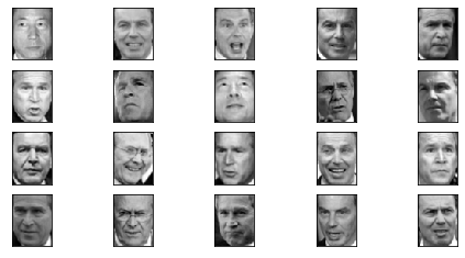
for i, ax in enumerate(axes.flat):ax.imshow(faces.images[i, :, :], cmap = 'gray')
fig
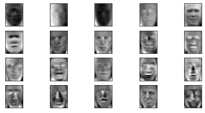
pca = PCA(150).fit(faces.data)
V = pca.components_
V.shape
(150, 2914)
V(k, n)乘原有的特征矩阵X,完成降维
fig, axes = plt.subplots(4, 5, figsize = [8, 4],subplot_kw = {'xticks':[], 'yticks':[]} # 不显示坐标轴)for i, ax in enumerate(axes.flat):ax.imshow(V[i, :].reshape(62, 47), cmap = 'gray')
x_tran = pca.transform(faces.data)
x_tran.shape
(964, 150)
5. inverse_transform
import matplotlib.pyplot as plt%matplotlib inlineimport numpy as npimport pandas as pdfrom sklearn.datasets import fetch_lfw_peoplefrom sklearn.decomposition import PCA
faces = fetch_lfw_people(min_faces_per_person = 60)
faces.data
array([[ 50.666668, 62. , 90.333336, ..., 68.666664, 78. ,80.333336],[117.666664, 106.666664, 96. , ..., 233.66667 , 234.33333 ,227. ],[ 70.666664, 64. , 58.666668, ..., 115. , 118. ,121.333336],...,[139. , 148.33333 , 156.33333 , ..., 49. , 19.333334,12. ],[126.666664, 118.666664, 133. , ..., 68.333336, 64.666664,56. ],[ 65.333336, 86. , 105.666664, ..., 179. , 93.333336,10.333333]], dtype=float32)
faces.data.shape
(964, 2914)
faces.images.shape
(964, 62, 47)
pca = PCA(150) # 实例化x_dr = pca.fit_transform(daces.data) # 拟合 + 提取结果
x_dr
array([[ -687.52765 , 658.6859 , -224.83125 , ..., -5.8305807,37.9641 , -68.2529 ],[ -520.3875 , -337.95184 , -85.0649 , ..., 56.23444 ,-7.104003 , -27.09345 ],[ -668.42316 , 177.38837 , 705.5544 , ..., -93.13145 ,-28.745838 , 41.614784 ],...,[-1426.5477 , -316.7213 , -184.77708 , ..., 73.25698 ,-9.299059 , -5.395314 ],[ 1393.6271 , 936.3961 , 599.951 , ..., 38.447098 ,25.35701 , -42.811676 ],[ 784.0877 , 469.102 , -400.20416 , ..., -21.948296 ,47.49396 , -11.908577 ]], dtype=float32)
x_dr.shape
(964, 150)
pca.explained_variance_ratio_.sum()
0.9528588
x_inverse = pca.inverse_transform(x_dr)
x_inverse
array([[ 61.003284 , 65.75134 , 73.682495 , ..., 67.226166 ,68.544495 , 72.683105 ],[102.78923 , 107.009964 , 110.27441 , ..., 233.90904 ,227.82428 , 215.0698 ],[ 65.36822 , 59.9917 , 58.116863 , ..., 113.183395 ,105.91263 , 102.84451 ],...,[124.8531 , 130.30939 , 145.5615 , ..., 73.5932 ,26.662682 , -2.8888931],[144.30975 , 138.76814 , 135.97636 , ..., 79.788666 ,65.55131 , 53.822388 ],[ 89.81032 , 98.244835 , 114.291756 , ..., 156.79715 ,75.214355 , 12.275055 ]], dtype=float32)
x_inverse.shape
(964, 2914)
fig, axes = plt.subplots(2, 10, figsize = (10, 2.5),subplot_kw = {'xticks':[], 'yticks':[]} # 不显示坐标轴)for i in range(10):axes[0, i].imshow(faces.images[i], cmap = 'binary_r')axes[1, i].imshow(x_inverse[i].reshape(62, 47), cmap = 'binary_r')
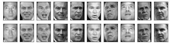
- fit_transform,降维
(964, 2914)—>(964, 150)
- inverse_transform,不是复原,而是将被降维的数据升维
(964, 150)—>(964, 2914) 能在多大程度上恢复原有的信息,取决于第一步降维时舍弃的信息量
- reshape
(964, 2914)—>(964, 62, 47)
用PCA过滤噪音
使用inverse_transform保持维度,去掉噪音
from sklearn.datasets import load_digits
查看原始数据图像
load_digits = load_digits()
load_digits.data.shape # 1797个样本,64个特征
(1797, 64)
load_digits.images.shape # 手写数字的本质是图像
(1797, 8, 8)
set(load_digits.target) # load_digits为手写数字识别数据,标签为0到9这十个数字
{0, 1, 2, 3, 4, 5, 6, 7, 8, 9}
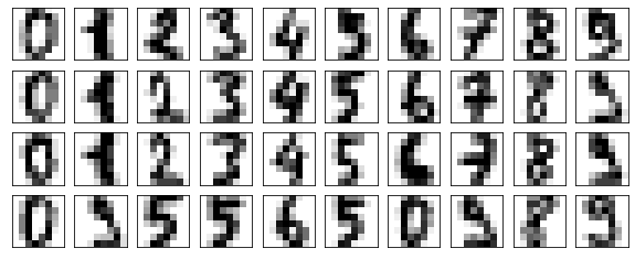
def plot_digits(data):# data的结构必须为 (m, n),且 n 可被分为 (x, y) 的像素结构fig, axes = plt.subplots(4 ,10, figsize = (10, 4),subplot_kw = {'xticks':[], 'yticks':[]})for i, ax in enumerate(axes.flat):ax.imshow(data[i].reshape(8, 8) # 若输入images数据,则不需要reshape, cmap = 'binary')
plot_digits(load_digits.images)
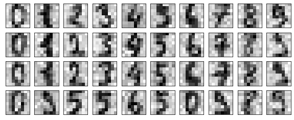
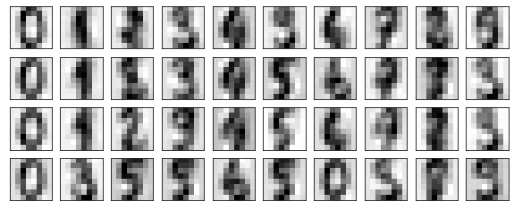
添加噪音
rng = np.random.RandomState(42)noisy = rng.normal(load_digits.data # 从原数据集中抽取正态分布的数据, 2 # 产生的新数据集的方差为2)noisy.shape
(1797, 64)
plot_digits(noisy)
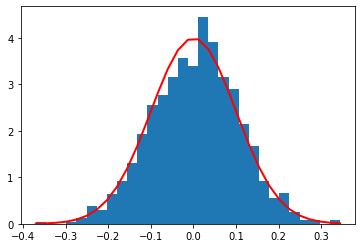
np.random.normal()的用法
loc:float 此概率分布的均值(对应着整个分布的中心centre)
scale:float 此概率分布的标准差(对应于分布的宽度,scale越大越矮胖,scale越小,越瘦高)
size:int or tuple of ints 输出的shape,默认为None,只输出一个值
概率密度函数:f(x)=\frac{1}{\sqrt{2π}\sigma}e2}{2\sigma^2}}
# 采样:s = rng.normal(loc=0, scale=.1, size=1000)# 拟合:count, bins, _ = plt.hist(s, 30, normed=True)# normed是进行拟合的关键# count统计某一bin出现的次数,在Normed为True时,可能其值会略有不同plt.plot(bins, 1./(np.sqrt(2*np.pi)*.1)*np.exp(-(bins-0)**2/(2*.1**2)), lw=2, c='r')
C:\anaconda\lib\site-packages\ipykernel_launcher.py:5: MatplotlibDeprecationWarning:The 'normed' kwarg was deprecated in Matplotlib 2.1 and will be removed in 3.1. Use 'density' instead."""[<matplotlib.lines.Line2D at 0x1442765a898>]
pca = PCA(0.5).fit(noisy)x_dr = pca.transform(noisy)x_dr.shape
(1797, 6)
x_inverse = pca.inverse_transform(x_dr)x_inverse.shape
(1797, 64)
plot_digits(x_inverse)
6. 案例:PCA对手写数据集的降维
from sklearn.ensemble import RandomForestClassifier as RFCfrom sklearn.model_selection import cross_val_score
data = pd.read_csv('digit recognizor.csv')data.shape
(42000, 785)
data.info()
<class 'pandas.core.frame.DataFrame'>RangeIndex: 42000 entries, 0 to 41999Columns: 785 entries, label to pixel783dtypes: int64(785)memory usage: 251.5 MB
data.head()
| label | pixel0 | pixel1 | pixel2 | pixel3 | pixel4 | pixel5 | pixel6 | pixel7 | pixel8 | … | pixel774 | pixel775 | pixel776 | pixel777 | pixel778 | pixel779 | pixel780 | pixel781 | pixel782 | pixel783 | |
|---|---|---|---|---|---|---|---|---|---|---|---|---|---|---|---|---|---|---|---|---|---|
| 0 | 1 | 0 | 0 | 0 | 0 | 0 | 0 | 0 | 0 | 0 | … | 0 | 0 | 0 | 0 | 0 | 0 | 0 | 0 | 0 | 0 |
| 1 | 0 | 0 | 0 | 0 | 0 | 0 | 0 | 0 | 0 | 0 | … | 0 | 0 | 0 | 0 | 0 | 0 | 0 | 0 | 0 | 0 |
| 2 | 1 | 0 | 0 | 0 | 0 | 0 | 0 | 0 | 0 | 0 | … | 0 | 0 | 0 | 0 | 0 | 0 | 0 | 0 | 0 | 0 |
| 3 | 4 | 0 | 0 | 0 | 0 | 0 | 0 | 0 | 0 | 0 | … | 0 | 0 | 0 | 0 | 0 | 0 | 0 | 0 | 0 | 0 |
| 4 | 0 | 0 | 0 | 0 | 0 | 0 | 0 | 0 | 0 | 0 | … | 0 | 0 | 0 | 0 | 0 | 0 | 0 | 0 | 0 | 0 |
5 rows × 785 columns
data.columns
Index(['label', 'pixel0', 'pixel1', 'pixel2', 'pixel3', 'pixel4', 'pixel5','pixel6', 'pixel7', 'pixel8',...'pixel774', 'pixel775', 'pixel776', 'pixel777', 'pixel778', 'pixel779','pixel780', 'pixel781', 'pixel782', 'pixel783'],dtype='object', length=785)
y = data.iloc[:, 0]x = data.iloc[:, 1:]x.shape
(42000, 784)
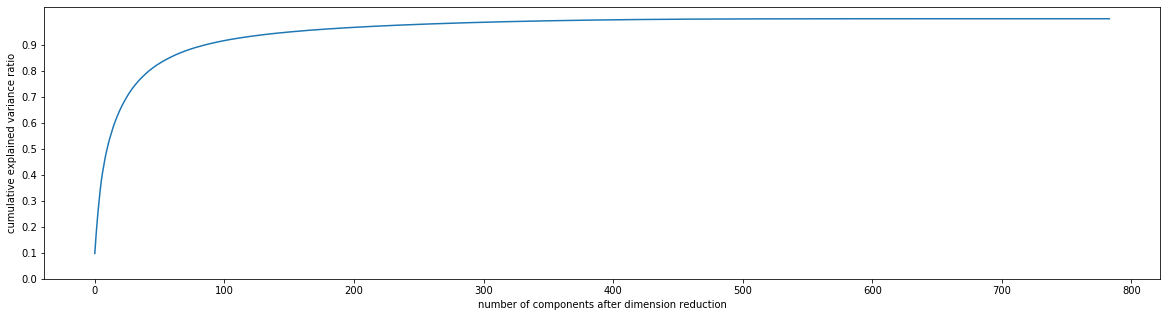
画累计方差贡献率曲线,找最佳的降维后维度的范围
pca_line = PCA().fit(x)plt.figure(figsize = (20, 5))plt.plot(np.cumsum(pca_line.explained_variance_ratio_))plt.xlabel('number of components after dimension reduction')plt.ylabel('cumulative explained variance ratio')plt.yticks(np.arange(0, 1, 0.1))
Text(0, 0.5, 'cumulative explained variance ratio')
画降维后的学习曲线,继续缩小最佳维度的范围
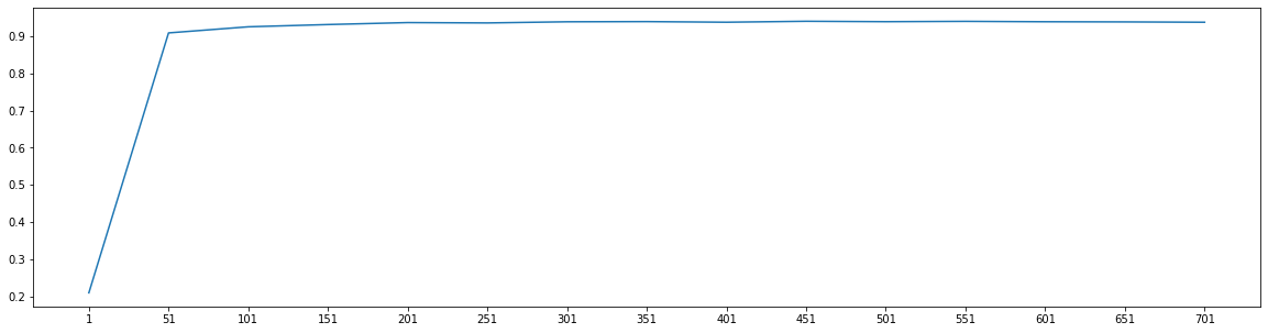
score = []for i in range(1, 101, 10):x_dr = PCA(i).fit_transform(x)once = cross_val_score(RFC(n_estimators = 10, random_state = 0), x_dr, y, cv =5).mean()score.append(once)plt.figure(figsize = (20, 5))plt.plot(score)
[<matplotlib.lines.Line2D at 0x14431964358>]
细化学习曲线,找出最佳降维维度
score = []for i in range(10, 25):x_dr = PCA(i).fit_transform(x)once = cross_val_score(RFC(n_estimators = 10, random_state = 0), x_dr, y, cv =5).mean()score.append(once)plt.figure(figsize = (20, 5))plt.plot(range(10, 25), score)
[<matplotlib.lines.Line2D at 0x14432c25240>]
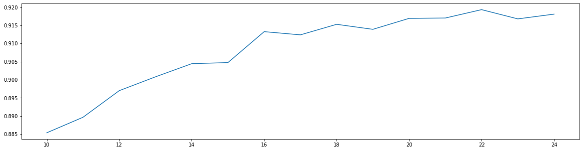
print(max(score), score.index(max(score)) + 10)
0.9193339375531199 22
导入最佳维度降维,查看模型效果
x_dr = PCA(22).fit_transform(x)score = cross_val_score(RFC(n_estimators = 100, random_state = 0), x_dr, y, cv =5).mean()score
0.9441668641981771
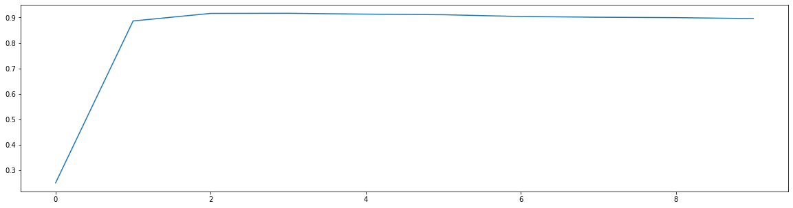
KNN的K值学习曲线
from sklearn.neighbors import KNeighborsClassifier as KNNx_dr = PCA(22).fit_transform(x)score = cross_val_score(KNN(), x_dr, y, cv =5).mean()score
0.9687611825661353
score = []for i in range(1, 11):x_dr = PCA(22).fit_transform(x)once = cross_val_score(KNN(i), x_dr, y, cv =5).mean()score.append(once)plt.figure(figsize = (20, 5))plt.plot(range(1, 11), score)
[<matplotlib.lines.Line2D at 0x144289b90f0>]
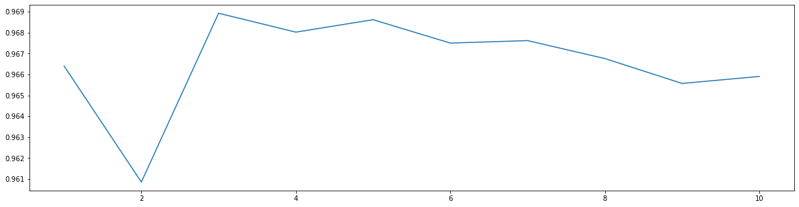
cross_val_score(KNN(3), x_dr, y, cv =5).mean()
0.969023172398515

若有收获,就点个赞吧
0 人点赞
