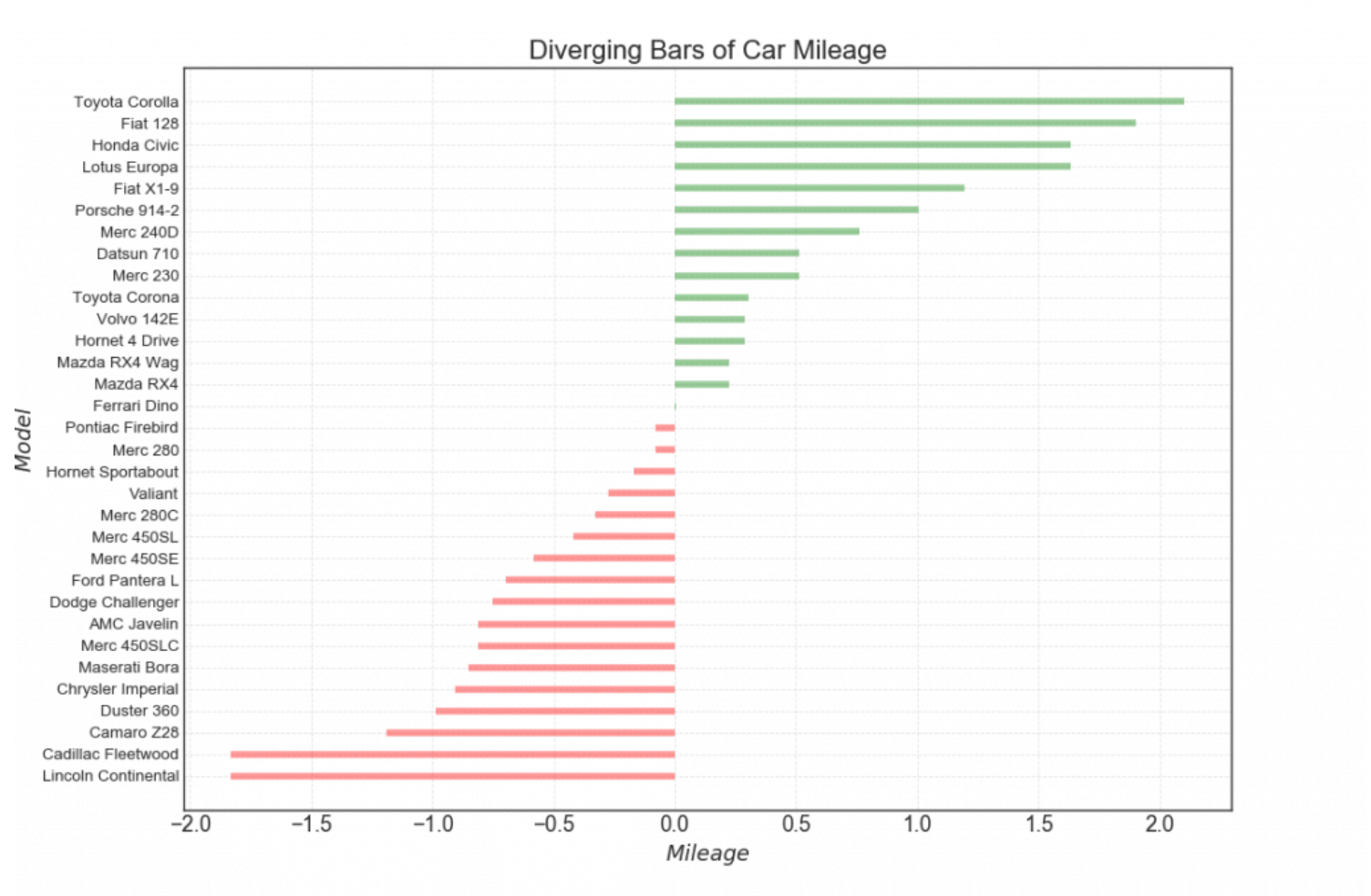
- 横坐标:里程
- 纵坐标:各品牌汽车
- 颜色:“<0”显示红色,“>0”显示绿色
1. 导入需要的绘图库
import numpy as npimport pandas as pdimport matplotlib.pyplot as plt%matplotlib inline
2. 绘制发散性条形图的函数
plt.hlines()
plt.hlines()绘制水平的条形图,类似的还有绘制垂直的条形图的plt.vlines()
参数说明:
y: y轴索引
xmin: 每行的开头
xmax: 每行的结尾
colors: 颜色,默认是‘k’(黑色)
linestyles : 线的类型,可选择{‘solid’, ‘dashed’, ‘dashdot’, ‘dotted’}
label: 标签,默认为空linewidth:线的宽度
alpha:色彩饱和度
X = np.random.rand(10)
plt.hlines(y = range(10), xmin = 0, xmax = X)
<matplotlib.collections.LineCollection at 0x2241b8856d8>
细节参数
与目标图像相比:
- 目标图像是从大到小顺序排列的
- 目标图像的线比较宽
- 目标图像是基于某个特定值将数据分为了两部分,并用不同颜色表示
(1) 让图像顺序排列
# 定义数据X = np.random.rand(10)
X
array([0.79320325, 0.3353483 , 0.4278299 , 0.35968898, 0.88311282,0.94948151, 0.84846223, 0.42299908, 0.81140851, 0.80943238])
方法一:
sorted(X, reverse = True) # 生成新的对象,不改变原数据
[0.9494815093607172,0.8831128154585404,0.8484622277078452,0.8114085082311853,0.8094323846159186,0.7932032509515197,0.42782989569642726,0.42299907682151494,0.35968897994232496,0.33534829671949107]
方法二:
X.sort() # 直接改变原数据
X
array([0.3353483 , 0.35968898, 0.42299908, 0.4278299 , 0.79320325,0.80943238, 0.81140851, 0.84846223, 0.88311282, 0.94948151])
# 绘图plt.hlines(y = range(10),xmin = 0, xmax = X # hlines()默认从下往上绘制)
<matplotlib.collections.LineCollection at 0x2241b936d68>
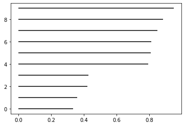
【注意】plt.hlines()的图像是从下往上依次画出的,.sort()返回的结果是从小到大排列,与图像从下往上的顺序吻合
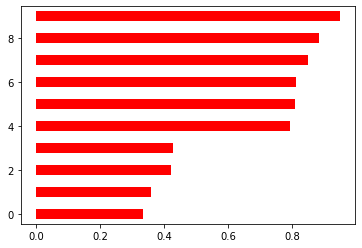
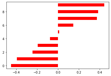
(2) 让线条宽一点
plt.hlines(y = range(10), xmin = 0, xmax = X, linewidth = 10, color = 'red')
<matplotlib.collections.LineCollection at 0x2241b99bc88>
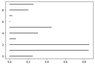
(3) 让图像基于均值分成两部分
# 定义数据X = np.random.rand(10)# 均值变为0X = X - X.mean()# 排序X.sort()
X
array([-0.4498374 , -0.3924608 , -0.24409046, -0.19477768, -0.07719991,0.0107024 , 0.14560278, 0.3734311 , 0.38530848, 0.4433215 ])
plt.hlines(y = range(10), xmin = 0, xmax = X, linewidth = 10, color = 'red')
<matplotlib.collections.LineCollection at 0x2241b9db5c0>
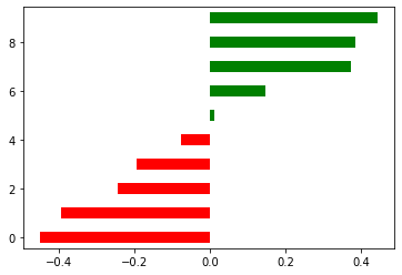
(4) 让图像两部分显示不同的颜色
plt.hlines(y = range(10), xmin = 0, xmax = X, linewidth = 10,color = ['red', 'red', 'red', 'red', 'red','green', 'green', 'green', 'green', 'green'])
<matplotlib.collections.LineCollection at 0x2241ba56dd8>
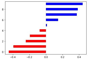
# 创建颜色列表colors = []for i in X:if i < 0:colors.append('red')else:colors.append('blue')
colors
['red', 'red', 'red', 'red', 'red', 'blue', 'blue', 'blue', 'blue', 'blue']
plt.hlines(y = range(10), xmin = 0, xmax = X, linewidth = 10,color = colors)
<matplotlib.collections.LineCollection at 0x2241bab5a90>
# 列表推导式写color参数plt.hlines(y = range(10), xmin = 0, xmax = X, linewidth = 10,color = ['red' if i < 0 else 'green' for i in X])
<matplotlib.collections.LineCollection at 0x2241bb137f0>

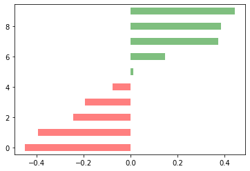
(5) 让颜色变浅一点
参数alpha是颜色饱和度,默认值为1
alpha取值范围是[0,1],越接近1颜色越饱和,也就是颜色越艳丽
plt.hlines(y = range(10), xmin = 0, xmax = X, linewidth = 10,color = ['red' if i < 0 else 'green' for i in X],alpha = 0.5)
<matplotlib.collections.LineCollection at 0x2241bb72278>
3. 认识绘图数据集
df = pd.read_csv('mtcars.csv')
df.shape
(32, 14)
df.info()
<class 'pandas.core.frame.DataFrame'>RangeIndex: 32 entries, 0 to 31Data columns (total 14 columns):mpg 32 non-null float64cyl 32 non-null int64disp 32 non-null float64hp 32 non-null int64drat 32 non-null float64wt 32 non-null float64qsec 32 non-null float64vs 32 non-null int64am 32 non-null int64gear 32 non-null int64carb 32 non-null int64fast 32 non-null int64cars 32 non-null objectcarname 32 non-null objectdtypes: float64(5), int64(7), object(2)memory usage: 3.6+ KB
sum(df.cars == df.carname)
32
sum(df.cars != df.carname)
0
df.columns
Index(['mpg', 'cyl', 'disp', 'hp', 'drat', 'wt', 'qsec', 'vs', 'am', 'gear','carb', 'fast', 'cars', 'carname'],dtype='object')
df.head()
| mpg | cyl | disp | hp | drat | wt | qsec | vs | am | gear | carb | fast | cars | carname | |
|---|---|---|---|---|---|---|---|---|---|---|---|---|---|---|
| 0 | 4.582576 | 6 | 160.0 | 110 | 3.90 | 2.620 | 16.46 | 0 | 1 | 4 | 4 | 1 | Mazda RX4 | Mazda RX4 |
| 1 | 4.582576 | 6 | 160.0 | 110 | 3.90 | 2.875 | 17.02 | 0 | 1 | 4 | 4 | 1 | Mazda RX4 Wag | Mazda RX4 Wag |
| 2 | 4.774935 | 4 | 108.0 | 93 | 3.85 | 2.320 | 18.61 | 1 | 1 | 4 | 1 | 1 | Datsun 710 | Datsun 710 |
| 3 | 4.626013 | 6 | 258.0 | 110 | 3.08 | 3.215 | 19.44 | 1 | 0 | 3 | 1 | 1 | Hornet 4 Drive | Hornet 4 Drive |
| 4 | 4.324350 | 8 | 360.0 | 175 | 3.15 | 3.440 | 17.02 | 0 | 0 | 3 | 2 | 1 | Hornet Sportabout | Hornet Sportabout |
所用数据集mtcars 记录了32种不同品牌的轿车的14个属性,如下所示:
mpg:英里每加仑(Miles per gallon) 值越大性能越好,或许是能源利用效率更高,或许速度较快
cyl:气缸数量(Number of cylinders)
disp:排量(Displacement)
hp:总马力(horsepower)
drat:驱动轴比(drive axle ratio)
wt:重量(Weight (lb/1000))
qsec:1/4英里所用时间(quarter mile time(secend))
vs:引擎(0-V shape,1-straight)
am:变速器(Transmission,0-automatic,1-manual)
gear:前进档数(Number of forward gears) #除了倒挡之外还有几个档
carb:化油器数量(Number of carburetors) #内燃机中用于混合空气和液体燃料的精细喷雾的装置。
fast: 用油是否高效(mpg>4 即为1,反之为0)
cars:汽车名称
carname:汽车名称(与cars完全相同)
绘制目标图所需的特征:
横坐标mileage指的是里程,所以可以推断所需要的特征就是mpg(消耗每加仑油跑多少英里)
纵坐标model指的是汽车的种类,所以直接用汽车名称cars或者caname都可以
df.mpg.values
array([4.58257569, 4.58257569, 4.77493455, 4.6260134 , 4.32434966,4.25440948, 3.78153408, 4.93963561, 4.77493455, 4.38178046,4.21900462, 4.04969135, 4.15932687, 3.89871774, 3.2249031 ,3.2249031 , 3.8340579 , 5.69209979, 5.5136195 , 5.82237065,4.63680925, 3.93700394, 3.89871774, 3.64691651, 4.38178046,5.22494019, 5.09901951, 5.5136195 , 3.97492138, 4.4384682 ,3.87298335, 4.6260134 ])
df.cars.values
array(['Mazda RX4', 'Mazda RX4 Wag', 'Datsun 710', 'Hornet 4 Drive','Hornet Sportabout', 'Valiant', 'Duster 360', 'Merc 240D','Merc 230', 'Merc 280', 'Merc 280C', 'Merc 450SE', 'Merc 450SL','Merc 450SLC', 'Cadillac Fleetwood', 'Lincoln Continental','Chrysler Imperial', 'Fiat 128', 'Honda Civic', 'Toyota Corolla','Toyota Corona', 'Dodge Challenger', 'AMC Javelin', 'Camaro Z28','Pontiac Firebird', 'Fiat X1-9', 'Porsche 914-2', 'Lotus Europa','Ford Pantera L', 'Ferrari Dino', 'Maserati Bora', 'Volvo 142E'],dtype=object)
# 添加画布,设置画布大小plt.figure(figsize = (12, 8))# 绘图plt.hlines(y = df.cars, xmin = 0, xmax = df.mpg,linewidth = 5, color = 'b', alpha = .5);
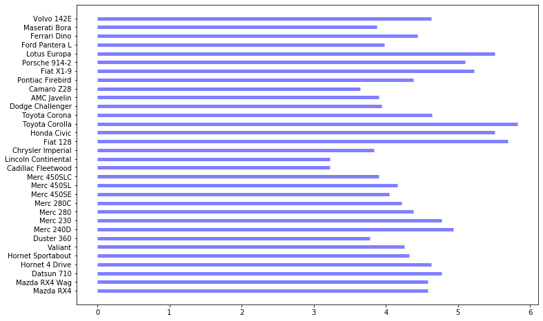
从这张图中,能看出的信息很少:
- 每种汽车的里程数
- 不同种类汽车里程数的相对大小
4. 对目标数据进行格式变换
提取目标数据并进行标准化处理
# 提取出mpg这一列的所有数据x = df.loc[:, 'mpg']# 采用z-score对目标数据进行标准化处理df['mpg_z'] = (x - x.mean())/x.std()
只是将原始数据进行了线性变换,并没有改变一个数据在该数据集中的位置
也没有改变该组数据的分布,而只是将均值变为0,标准差变为1
df.head()
| mpg | cyl | disp | hp | drat | wt | qsec | vs | am | gear | carb | fast | cars | carname | mpg_z | |
|---|---|---|---|---|---|---|---|---|---|---|---|---|---|---|---|
| 0 | 4.582576 | 6 | 160.0 | 110 | 3.90 | 2.620 | 16.46 | 0 | 1 | 4 | 4 | 1 | Mazda RX4 | Mazda RX4 | 0.223563 |
| 1 | 4.582576 | 6 | 160.0 | 110 | 3.90 | 2.875 | 17.02 | 0 | 1 | 4 | 4 | 1 | Mazda RX4 Wag | Mazda RX4 Wag | 0.223563 |
| 2 | 4.774935 | 4 | 108.0 | 93 | 3.85 | 2.320 | 18.61 | 1 | 1 | 4 | 1 | 1 | Datsun 710 | Datsun 710 | 0.514515 |
| 3 | 4.626013 | 6 | 258.0 | 110 | 3.08 | 3.215 | 19.44 | 1 | 0 | 3 | 1 | 1 | Hornet 4 Drive | Hornet 4 Drive | 0.289265 |
| 4 | 4.324350 | 8 | 360.0 | 175 | 3.15 | 3.440 | 17.02 | 0 | 0 | 3 | 2 | 1 | Hornet Sportabout | Hornet Sportabout | -0.167015 |
生成颜色标签
df['colors'] = ['red' if i < 0 else 'green' for i in df.mpg_z]
df.head()
| mpg | cyl | disp | hp | drat | wt | qsec | vs | am | gear | carb | fast | cars | carname | mpg_z | colors | |
|---|---|---|---|---|---|---|---|---|---|---|---|---|---|---|---|---|
| 0 | 4.582576 | 6 | 160.0 | 110 | 3.90 | 2.620 | 16.46 | 0 | 1 | 4 | 4 | 1 | Mazda RX4 | Mazda RX4 | 0.223563 | green |
| 1 | 4.582576 | 6 | 160.0 | 110 | 3.90 | 2.875 | 17.02 | 0 | 1 | 4 | 4 | 1 | Mazda RX4 Wag | Mazda RX4 Wag | 0.223563 | green |
| 2 | 4.774935 | 4 | 108.0 | 93 | 3.85 | 2.320 | 18.61 | 1 | 1 | 4 | 1 | 1 | Datsun 710 | Datsun 710 | 0.514515 | green |
| 3 | 4.626013 | 6 | 258.0 | 110 | 3.08 | 3.215 | 19.44 | 1 | 0 | 3 | 1 | 1 | Hornet 4 Drive | Hornet 4 Drive | 0.289265 | green |
| 4 | 4.324350 | 8 | 360.0 | 175 | 3.15 | 3.440 | 17.02 | 0 | 0 | 3 | 2 | 1 | Hornet Sportabout | Hornet Sportabout | -0.167015 | red |
df['colors'].value_counts()
red 17green 15Name: colors, dtype: int64
对数据集排序
原数据是无序排列的,需要对数据进行排序
这里需要注意的是,不止要对x进行排序,还需要确保y索引跟着一起变化,所以应该对整个数据集进行排序
df.sort_values('mpg_z', inplace = True)
df.head()
| mpg | cyl | disp | hp | drat | wt | qsec | vs | am | gear | carb | fast | cars | carname | mpg_z | colors | |
|---|---|---|---|---|---|---|---|---|---|---|---|---|---|---|---|---|
| 15 | 3.224903 | 8 | 460.0 | 215 | 3.00 | 5.424 | 17.82 | 0 | 0 | 3 | 4 | 0 | Lincoln Continental | Lincoln Continental | -1.829979 | red |
| 14 | 3.224903 | 8 | 472.0 | 205 | 2.93 | 5.250 | 17.98 | 0 | 0 | 3 | 4 | 0 | Cadillac Fleetwood | Cadillac Fleetwood | -1.829979 | red |
| 23 | 3.646917 | 8 | 350.0 | 245 | 3.73 | 3.840 | 15.41 | 0 | 0 | 3 | 4 | 0 | Camaro Z28 | Camaro Z28 | -1.191664 | red |
| 6 | 3.781534 | 8 | 360.0 | 245 | 3.21 | 3.570 | 15.84 | 0 | 0 | 3 | 4 | 0 | Duster 360 | Duster 360 | -0.988049 | red |
| 16 | 3.834058 | 8 | 440.0 | 230 | 3.23 | 5.345 | 17.42 | 0 | 0 | 3 | 4 | 0 | Chrysler Imperial | Chrysler Imperial | -0.908604 | red |
# 排序之后索引也会跟着一起打乱,需要重置索引df.reset_index(drop = True, inplace = True)
df.head()
| mpg | cyl | disp | hp | drat | wt | qsec | vs | am | gear | carb | fast | cars | carname | mpg_z | colors | |
|---|---|---|---|---|---|---|---|---|---|---|---|---|---|---|---|---|
| 0 | 3.224903 | 8 | 460.0 | 215 | 3.00 | 5.424 | 17.82 | 0 | 0 | 3 | 4 | 0 | Lincoln Continental | Lincoln Continental | -1.829979 | red |
| 1 | 3.224903 | 8 | 472.0 | 205 | 2.93 | 5.250 | 17.98 | 0 | 0 | 3 | 4 | 0 | Cadillac Fleetwood | Cadillac Fleetwood | -1.829979 | red |
| 2 | 3.646917 | 8 | 350.0 | 245 | 3.73 | 3.840 | 15.41 | 0 | 0 | 3 | 4 | 0 | Camaro Z28 | Camaro Z28 | -1.191664 | red |
| 3 | 3.781534 | 8 | 360.0 | 245 | 3.21 | 3.570 | 15.84 | 0 | 0 | 3 | 4 | 0 | Duster 360 | Duster 360 | -0.988049 | red |
| 4 | 3.834058 | 8 | 440.0 | 230 | 3.23 | 5.345 | 17.42 | 0 | 0 | 3 | 4 | 0 | Chrysler Imperial | Chrysler Imperial | -0.908604 | red |
5. 绘制目标图形
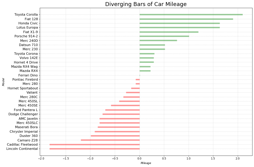
plt.figure(figsize = (14, 10))plt.hlines(y = df.cars, xmin = 0, xmax = df.mpg_z,color = df.colors, linewidth = 5, alpha = .6)plt.ylabel('$Model$', fontsize = 15)plt.xlabel('$Mileage$', fontsize = 15)plt.yticks(fontsize = 12)plt.title('Diverging Bars of Car Mileage', fontdict = {'size':20, 'color':'k'})plt.grid(linestyle = '--', alpha = .5)
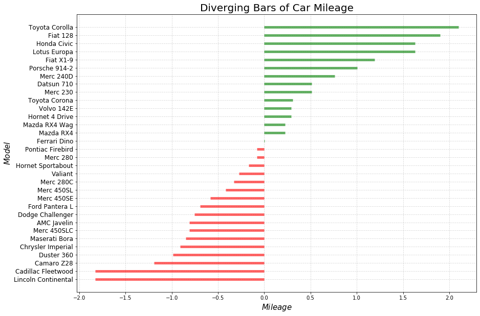
# 原始代码# Prepare Datadf = pd.read_csv("mtcars.csv") #导入数据集x = df.loc[:, ['mpg']] #提取目标数据df['mpg_z'] = (x - x.mean())/x.std() #对目标数据进行z-score标准化处理df['colors'] = ['red' if x < 0 else 'green' for x in df['mpg_z']] #生成颜色标签列df.sort_values('mpg_z', inplace=True) #根据标准化后的数据对整个数据集进行排序df.reset_index(inplace=True) #重置数据集的索引(这里是新增加了一列索引)# Draw plotplt.figure(figsize=(14,10), dpi= 65) #创建画布并设置画布大小plt.hlines(y=df.index, xmin=0, xmax=df.mpg_z, color=df.colors, alpha=0.4, linewidth=5)#绘制基础图形# Decorationsplt.gca().set(ylabel='$Model$', xlabel='$Mileage$')#get current axes,获取当前子图,若果没有子图则创建一个子图,并设置横纵轴名称plt.yticks(df.index, df.cars, fontsize=12) #将y轴刻度标签修改为汽车名称,并设置字体大小plt.title('Diverging Bars of Car Mileage', fontdict={'size':20}) #添加图标标题,并设置标题字体大小plt.grid(linestyle='--', alpha=0.5) #配置网格线plt.show() #本地显示图像
6. 图形解读
(1)相同油耗内里程数最小的是林肯大陆 (Lincoln Continental)
这款车一开始是福特汽车公司总裁Edsel Ford的私人车辆
从1939年至今已经更新十代
林肯系列车走的是高端路线,油耗里程已经不再是它关注的重点
(2)位于均值线上的是法拉利迪诺(Ferrari Dino)
“Dino”品牌的诞生是为了推出一款价格较低,“价格合理”的跑车
“Dino”这个名字是为了纪念这位创始人已故的儿子Alfredo Dino Ferrari,他因设计用于汽车的V6发动机而受到赞誉
(3)油耗里程数最大的是丰田卡罗拉(Toyota Corolla)
这是丰田生产的一系列超小型和紧凑型轿车
从1966年至今,已经更新十二代
卡罗拉于1966年推出,是1974年全球最畅销的汽车,自那时起成为全球最畅销的汽车之一
(4)从图形上来看,这32款汽车根据相同油耗内的里程数被分成了两组
一组高于平均值,从图中可以看出基本上都是一些民用车(除了那款保时捷914之外)
一组低于平均值,基本上都是高端车,要不就是跑车,要不就是商用车
(5)大胆猜想:发散型条形图完成了聚类功能
7. 用Kmeans聚类验证发散型条形图聚类效果
7.1 根据发散型条形图结果给原数据集添加标签
df.head()
| index | mpg | cyl | disp | hp | drat | wt | qsec | vs | am | gear | carb | fast | cars | carname | mpg_z | colors | |
|---|---|---|---|---|---|---|---|---|---|---|---|---|---|---|---|---|---|
| 0 | 15 | 3.224903 | 8 | 460.0 | 215 | 3.00 | 5.424 | 17.82 | 0 | 0 | 3 | 4 | 0 | Lincoln Continental | Lincoln Continental | -1.829979 | red |
| 1 | 14 | 3.224903 | 8 | 472.0 | 205 | 2.93 | 5.250 | 17.98 | 0 | 0 | 3 | 4 | 0 | Cadillac Fleetwood | Cadillac Fleetwood | -1.829979 | red |
| 2 | 23 | 3.646917 | 8 | 350.0 | 245 | 3.73 | 3.840 | 15.41 | 0 | 0 | 3 | 4 | 0 | Camaro Z28 | Camaro Z28 | -1.191664 | red |
| 3 | 6 | 3.781534 | 8 | 360.0 | 245 | 3.21 | 3.570 | 15.84 | 0 | 0 | 3 | 4 | 0 | Duster 360 | Duster 360 | -0.988049 | red |
| 4 | 16 | 3.834058 | 8 | 440.0 | 230 | 3.23 | 5.345 | 17.42 | 0 | 0 | 3 | 4 | 0 | Chrysler Imperial | Chrysler Imperial | -0.908604 | red |
df['label'] = [1 if i == 'red' else 0 for i in df.colors]
df.drop('index', axis = 1, inplace = True)
df.head()
| mpg | cyl | disp | hp | drat | wt | qsec | vs | am | gear | carb | fast | cars | carname | mpg_z | colors | label | |
|---|---|---|---|---|---|---|---|---|---|---|---|---|---|---|---|---|---|
| 0 | 3.224903 | 8 | 460.0 | 215 | 3.00 | 5.424 | 17.82 | 0 | 0 | 3 | 4 | 0 | Lincoln Continental | Lincoln Continental | -1.829979 | red | 1 |
| 1 | 3.224903 | 8 | 472.0 | 205 | 2.93 | 5.250 | 17.98 | 0 | 0 | 3 | 4 | 0 | Cadillac Fleetwood | Cadillac Fleetwood | -1.829979 | red | 1 |
| 2 | 3.646917 | 8 | 350.0 | 245 | 3.73 | 3.840 | 15.41 | 0 | 0 | 3 | 4 | 0 | Camaro Z28 | Camaro Z28 | -1.191664 | red | 1 |
| 3 | 3.781534 | 8 | 360.0 | 245 | 3.21 | 3.570 | 15.84 | 0 | 0 | 3 | 4 | 0 | Duster 360 | Duster 360 | -0.988049 | red | 1 |
| 4 | 3.834058 | 8 | 440.0 | 230 | 3.23 | 5.345 | 17.42 | 0 | 0 | 3 | 4 | 0 | Chrysler Imperial | Chrysler Imperial | -0.908604 | red | 1 |
7.2 利用Kmeans算法对原数据集进行聚类
from sklearn.cluster import KMeans
df1 = pd.read_csv('mtcars.csv')
df1.head()
| mpg | cyl | disp | hp | drat | wt | qsec | vs | am | gear | carb | fast | cars | carname | |
|---|---|---|---|---|---|---|---|---|---|---|---|---|---|---|
| 0 | 4.582576 | 6 | 160.0 | 110 | 3.90 | 2.620 | 16.46 | 0 | 1 | 4 | 4 | 1 | Mazda RX4 | Mazda RX4 |
| 1 | 4.582576 | 6 | 160.0 | 110 | 3.90 | 2.875 | 17.02 | 0 | 1 | 4 | 4 | 1 | Mazda RX4 Wag | Mazda RX4 Wag |
| 2 | 4.774935 | 4 | 108.0 | 93 | 3.85 | 2.320 | 18.61 | 1 | 1 | 4 | 1 | 1 | Datsun 710 | Datsun 710 |
| 3 | 4.626013 | 6 | 258.0 | 110 | 3.08 | 3.215 | 19.44 | 1 | 0 | 3 | 1 | 1 | Hornet 4 Drive | Hornet 4 Drive |
| 4 | 4.324350 | 8 | 360.0 | 175 | 3.15 | 3.440 | 17.02 | 0 | 0 | 3 | 2 | 1 | Hornet Sportabout | Hornet Sportabout |
df1.mpg.values
array([4.58257569, 4.58257569, 4.77493455, 4.6260134 , 4.32434966,4.25440948, 3.78153408, 4.93963561, 4.77493455, 4.38178046,4.21900462, 4.04969135, 4.15932687, 3.89871774, 3.2249031 ,3.2249031 , 3.8340579 , 5.69209979, 5.5136195 , 5.82237065,4.63680925, 3.93700394, 3.89871774, 3.64691651, 4.38178046,5.22494019, 5.09901951, 5.5136195 , 3.97492138, 4.4384682 ,3.87298335, 4.6260134 ])
# 提取出目标数据,由于sklearn不接受一维数据,所以需要对目标数据进行变形(转置)data_x = df1.mpg.values.reshape(-1, 1)
# 执行聚类cluster = KMeans(n_clusters = 2, random_state = 0).fit(data_x)# n_clusters:聚类数量# random_state:随机数种子
cluster
KMeans(algorithm='auto', copy_x=True, init='k-means++', max_iter=300,n_clusters=2, n_init=10, n_jobs=None, precompute_distances='auto',random_state=0, tol=0.0001, verbose=0)
cluster.labels_
array([0, 0, 0, 0, 1, 1, 1, 0, 0, 1, 1, 1, 1, 1, 1, 1, 1, 0, 0, 0, 0, 1,1, 1, 1, 0, 0, 0, 1, 1, 1, 0])
# 新建一列标签列,将聚类的结果作为标签df1['label'] = cluster.labels_
df1.head()
| mpg | cyl | disp | hp | drat | wt | qsec | vs | am | gear | carb | fast | cars | carname | label | |
|---|---|---|---|---|---|---|---|---|---|---|---|---|---|---|---|
| 0 | 4.582576 | 6 | 160.0 | 110 | 3.90 | 2.620 | 16.46 | 0 | 1 | 4 | 4 | 1 | Mazda RX4 | Mazda RX4 | 0 |
| 1 | 4.582576 | 6 | 160.0 | 110 | 3.90 | 2.875 | 17.02 | 0 | 1 | 4 | 4 | 1 | Mazda RX4 Wag | Mazda RX4 Wag | 0 |
| 2 | 4.774935 | 4 | 108.0 | 93 | 3.85 | 2.320 | 18.61 | 1 | 1 | 4 | 1 | 1 | Datsun 710 | Datsun 710 | 0 |
| 3 | 4.626013 | 6 | 258.0 | 110 | 3.08 | 3.215 | 19.44 | 1 | 0 | 3 | 1 | 1 | Hornet 4 Drive | Hornet 4 Drive | 0 |
| 4 | 4.324350 | 8 | 360.0 | 175 | 3.15 | 3.440 | 17.02 | 0 | 0 | 3 | 2 | 1 | Hornet Sportabout | Hornet Sportabout | 1 |
【注意】
发散型条形图的数据 df 经过了排序,所以这里 df1 也需要将数据排序
需要保证的是两者排序的依据是一样的,都是根据mpg这个特征排序
df1.sort_values('mpg', inplace = True)
# 重置索引 方法一df1.reset_index(inplace = True)
df1.head()
| index | mpg | cyl | disp | hp | drat | wt | qsec | vs | am | gear | carb | fast | cars | carname | label | |
|---|---|---|---|---|---|---|---|---|---|---|---|---|---|---|---|---|
| 0 | 15 | 3.224903 | 8 | 460.0 | 215 | 3.00 | 5.424 | 17.82 | 0 | 0 | 3 | 4 | 0 | Lincoln Continental | Lincoln Continental | 1 |
| 1 | 14 | 3.224903 | 8 | 472.0 | 205 | 2.93 | 5.250 | 17.98 | 0 | 0 | 3 | 4 | 0 | Cadillac Fleetwood | Cadillac Fleetwood | 1 |
| 2 | 23 | 3.646917 | 8 | 350.0 | 245 | 3.73 | 3.840 | 15.41 | 0 | 0 | 3 | 4 | 0 | Camaro Z28 | Camaro Z28 | 1 |
| 3 | 6 | 3.781534 | 8 | 360.0 | 245 | 3.21 | 3.570 | 15.84 | 0 | 0 | 3 | 4 | 0 | Duster 360 | Duster 360 | 1 |
| 4 | 16 | 3.834058 | 8 | 440.0 | 230 | 3.23 | 5.345 | 17.42 | 0 | 0 | 3 | 4 | 0 | Chrysler Imperial | Chrysler Imperial | 1 |
df.head()
| mpg | cyl | disp | hp | drat | wt | qsec | vs | am | gear | carb | fast | cars | carname | mpg_z | colors | label | |
|---|---|---|---|---|---|---|---|---|---|---|---|---|---|---|---|---|---|
| 0 | 3.224903 | 8 | 460.0 | 215 | 3.00 | 5.424 | 17.82 | 0 | 0 | 3 | 4 | 0 | Lincoln Continental | Lincoln Continental | -1.829979 | red | 1 |
| 1 | 3.224903 | 8 | 472.0 | 205 | 2.93 | 5.250 | 17.98 | 0 | 0 | 3 | 4 | 0 | Cadillac Fleetwood | Cadillac Fleetwood | -1.829979 | red | 1 |
| 2 | 3.646917 | 8 | 350.0 | 245 | 3.73 | 3.840 | 15.41 | 0 | 0 | 3 | 4 | 0 | Camaro Z28 | Camaro Z28 | -1.191664 | red | 1 |
| 3 | 3.781534 | 8 | 360.0 | 245 | 3.21 | 3.570 | 15.84 | 0 | 0 | 3 | 4 | 0 | Duster 360 | Duster 360 | -0.988049 | red | 1 |
| 4 | 3.834058 | 8 | 440.0 | 230 | 3.23 | 5.345 | 17.42 | 0 | 0 | 3 | 4 | 0 | Chrysler Imperial | Chrysler Imperial | -0.908604 | red | 1 |
# 重置索引 方法二df1.index = range(df.shape[0])
7.3 计算准确率
sum(df.label == df1.label)/df.shape[0]
0.96875
(df.label == df1.label).mean()
0.96875
df1.label.values
array([1, 1, 1, 1, 1, 1, 1, 1, 1, 1, 1, 1, 1, 1, 1, 1, 1, 1, 0, 0, 0, 0,0, 0, 0, 0, 0, 0, 0, 0, 0, 0])
df.label.values
array([1, 1, 1, 1, 1, 1, 1, 1, 1, 1, 1, 1, 1, 1, 1, 1, 1, 0, 0, 0, 0, 0,0, 0, 0, 0, 0, 0, 0, 0, 0, 0], dtype=int64)
df[df.label != df1.label]
| mpg | cyl | disp | hp | drat | wt | qsec | vs | am | gear | carb | fast | cars | carname | mpg_z | colors | label | |
|---|---|---|---|---|---|---|---|---|---|---|---|---|---|---|---|---|---|
| 17 | 4.438468 | 6 | 145.0 | 175 | 3.62 | 2.77 | 15.5 | 0 | 1 | 5 | 6 | 1 | Ferrari Dino | Ferrari Dino | 0.005594 | green | 0 |

若有收获,就点个赞吧
0 人点赞
