greedy algorithm贪心法
概念
A greedy algorithm constructs a solution to the problem by always making a choice that looks the best at the moment. A greedy algorithm never takes back its choices, but directly constructs the final solution. For this reason, greedy algorithms are usually very efficient.
The difficulty in designing greedy algorithms is to find a greedy strategy that always produces an optimal solution to the problem. The locally optimal choices in a greedy algorithm should also be globally optimal. It is often difficult to argue that a greedy algorithm works.
每一步行动总是按某种指标选取最优的操作进行,该指标只看眼前,并不考虑可能造成的影响。可想而知,并不是所有的时候贪心法都能获得最优解,所以一般使用贪心法的时候,都要确保自己能证明其正确性。
Coin problem硬币问题
As a first example, we consider a problem where we are given a set of coins and our task is to form a sum of money n using the coins. The values of the coins are coins={c_1,_c_2,…,_ck}, and each coin can be used as many times we want. What is the minimum number of coins needed?
硬币的面值有{1, 2, 5, 10, 20, 50, 100, 200},如果要取得520元,我们至少需要4枚硬币。200+200+100+20 = 520
然而,贪心并不一直都是最佳方案。比如硬币的面值有{1, 3, 4},如果需要取得6元,使用贪心的思路,每一次取最大的,取的方案是{4, 1, 1},三枚硬币。然而,我们知道最佳方案是{3, 3},只需要两枚硬币。(这时,我们就会需要动态规划)
Scheduling时间安排问题
Given n events with their starting and ending times, find a schedule that includes as many events as possible.
event starting time ending timeA 1 3B 2 5C 3 9D 6 8
算法1
The first idea is to select as short events as possible. In the example case this algorithm selects the following events: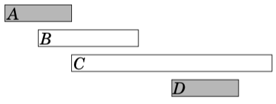
However, selecting short events is not always a correct strategy. For example, the algorithm fails in the following case: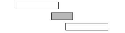
If we select the short event, we can only select one event. However, it would be possible to select both long events.
算法2
Another idea is to always select the next possible event that begins as early as possible. This algorithm selects the following events: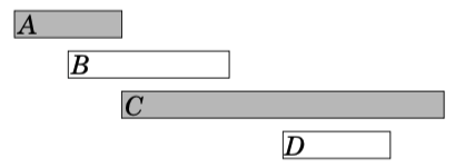
However, we can find a counter example also for this algorithm. For example, in the following case, the algorithm only selects one event: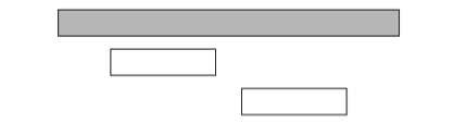
If we select the first event, it is not possible to select any other events. However, it would be possible to select the other two events.
算法3
The third idea is to always select the next possible event that ends as early as possible. This algorithm selects the following events: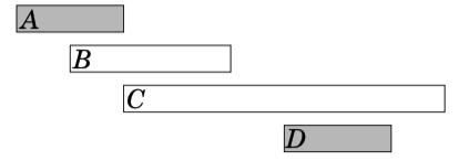
[证明]
It turns out that this algorithm always produces an optimal solution. The reason for this is that it is always an optimal choice to first select an event that ends as early as possible. After this, it is an optimal choice to select the next event using the same strategy, etc., until we cannot select any more events.
One way to argue that the algorithm works is to consider what happens if we first select an event that ends later than the event that ends as early as possible. Now, we will have at most an equal number of choices how we can select the next event. Hence, selecting an event that ends later can never yield a better solution, and the greedy algorithm is correct.
Tasks and deadlines任务截止时间问题
Let us now consider a problem where we are given n tasks with durations and deadlines and our task is to choose an order to perform the tasks. For each task, we earn d − x points where d is the task’s deadline and x is the moment when we finish the task. What is the largest possible total score we can obtain?
task duration deadlineA 4 2B 3 5C 2 7D 4 5
In this case, an optimal schedule for the tasks is as follows: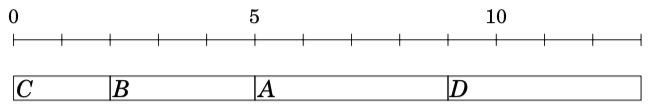
In this solution, C yields 5 points, B yields 0 points, A yields −7 points and D yields −8 points, so the total score is −10.
Surprisingly, the optimal solution to the problem does not depend on the deadlines at all, but a correct greedy strategy is to simply perform the tasks sorted by their durations in increasing order. The reason for this is that if we ever perform two tasks one after another such that the first task takes longer than the second task, we can obtain a better solution if we swap the tasks. For example, consider the following schedule: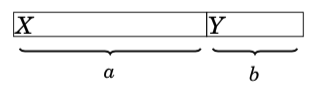
Here a > b, so we should swap the tasks: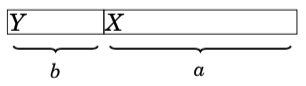
[证明]
Now X gives b points less and Y gives a points more, so the total score increases by a − b > 0. In an optimal solution, for any two consecutive tasks, it must hold that the shorter task comes before the longer task. Thus, the tasks must be performed sorted by their durations.(假设,右边边界是得分deadline,交换完之后,x得分少得了b分,y得到多了a分,a-b>0,总共会得更多的分数。所以,正确)
Minimizing sums求最小的和
We next consider a problem where we are given n numbers a_1,_a_2,…,_an and our task is to find a value x that minimizes the sum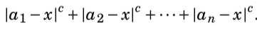
我们讨论一下,当 c = 1的情况 和 当 c = 2 的情况
当 c = 1的情况
|a1 - x| + |a2 - x| + ... + |an - x|
For example, if the numbers are [1, 2, 9, 2, 6], the best solution is to select x = 2 which produces the sum
|1 - 2| + |2 - 2| + |9 - 2| + |2 - 2| + |6 - 2| = 1 + 0 + 7 + 0 + 4 = 12
In the general case, the best choice for x is the median of the numbers, i.e., the middle number after sorting. For example, the list [1, 2, 9, 2, 6] becomes [1, 2, 2, 6, 9] after sorting, so the median is 2.
The median is an optimal choice, because if x is smaller than the median, the sum becomes smaller by increasing x, and if x is larger then the median, the sum becomes smaller by decreasing x. Hence, the optimal solution is that x is the median. If n is even and there are two medians, both medians and all values between them are optimal choices.
当 c = 2的情况
(a1 - x)^2 + (a2 - x)^2 + ... + (an - x)^2
For example, if the numbers are [1, 2, 9, 2, 6], the best solution is to select x = 4.
(1 - 4)^2 + (2 - 4)^2 + (9 - 4)^2 + (2 - 4)^2 + (6 - 4)^2 = 46
In the general case, the best choice for x is the average of the numbers. In the example the average is (1+2+9+2+6)/5 = 4.
The last part does not depend on x, so we can ignore it. The remaining parts form a function , where
  . This is a parabola opening upwards with roots x = 0 and x = 2s/n, and the minimum value is the average of the roots x = s/n, i.e., the average of the numbers a_1,_a_2,…,_an.
贪心常见题型
- 按某种顺序排序后,然后逐个取(sort,多关键字排序,重载小于符号)
- 每次取集合中的最大/最小,更新答案(使用priority_queue)
贪心在最优子结构的问题中尤为有效(最优子结构的意思是问题能够分解成子问题来解决,子问题的最优解能递推到最终问题的最优解。)
贪心与dp的区别,贪心对每个子问题的解决方案都做出选择,不能回退。dp会保存以前的运算结果,并根据以前的结果进行选择,有回退功能。
有的时候,贪心并不是正确的,比如01背包问题,贪心就会出错。贪心问题特别像逻辑题,方法很简单,但是证明却很难。考场上,不需要会证明。
贪心法证明的常见方法
- 反证法(假设、调整、做差)
- A>=B, A <= B, 证明A=B
- 数学归纳法
例题
例题,【例6.1】排队接水
//排序类型
例题,【例6.3】删数问题(Noip1994)
//贪心:干掉下降子序列第一个数字。或者模拟取找
例题,【例6.5】活动选择
//排序类型,数轴上的问题
例题,【例6.6】整数区间
//排序类型,数轴上的问题,会用到双指针方法
例题,最大子矩阵
//纯暴力会T,学习使用二维前缀和
recursion递推法
概念
学习使用递推的前提:一维数组,或者要会使用有限个变量,互相传递数值迭代前进的操作。
引言:一个实际问题的各种可能情况构成的集合,通常称为 “状态空间”,而程序的运行则是对状态空间的遍历。
递推 是程序遍历状态空间的基本方式。由已知的 “问题边界” 为起点,向 “原问题” 正向推导的扩展方式就是递推。
例子:询问有几个苹果,有每个人向上反馈,得到有n个苹果。
例子:Fibonacci数列
例子:兔子繁殖问题,把雌雄各一的一对新兔子放入养殖场中。每只雌兔在出生两个月以后,每月产雌雄各一的一对新兔子。试问,第n个月后养殖场中有多少对兔子。
- 请编程实现一下,兔子繁殖问题,输出前10个月兔子的数量,每行一个数字
- 理解兔子繁殖问题的时候,不建议画很繁杂的图,会容易扰乱思考
- 集合划分方法,分析出递推公式,上个月就有的老兔子 + 这个月出生的新兔子
f(n) = f(n - 1) + f(n - 2)例题
例题,上台阶
//简单
例题,菲波那契数列(2)
//简单
例题,Pell数列
//简单
例题,【例3.4】昆虫繁殖
//用一个数组维护成虫数量,用一个数组维护卵的数量//不开long long见祖宗
例题,流感传染
//模拟,一层一层的扩大感染的范围//注意这个扩散是一层一层的扩散,要注意控制这个一层一层的问题,需要用到标记数组
例题,放苹果
```cpp //这个理解有难度,分为 //盘子比苹果多的情况,苹果比盘子多的情况
// 苹果的数量比盘子多的时候: // 有空盘子,那至少应该有一个盘子剩余:f(m,n-1) // 没有空盘子,那至少每一个盘子都有一个苹果,去掉n个苹果也是多放法总数不构成影响:f(m-n,n) // 盘子的数量比苹果的时候: // 去掉多余的盘子对摆放不构成影响:f(m, m)
// 问题边界 // 手里有0个苹果,就1种放法。(如果手里有1个苹果,这个方法并不唯一,如果面临现有盘子里苹果数量不一样) // 有1个盘子时候,也只有1种放法,就是有苹果就放这个盘子,没苹果就不放
<a name="KKWzd"></a># recursive递归法<a name="eRCWu"></a>## 概念> **学习使用递归的前提:**> 函数理解深入(带参的函数,有返回值的函数,函数的嵌套(就是“自身调用自身”))> 操作时,试验无限递归> 递归的终止条件> “回溯时还原现场”保证执行前后程序面对问题的状态是相同的。递归是程序遍历状态空间的基本方式。<br />以“原问题”为起点,尝试寻找把状态空间缩小到已知的“问题边界”的路线。<br />再通过该路线反向回溯的遍历方式,就是递归。程序在每个步骤应该面对相同种类的问题,这些问题都是原问题的一个子问题,可能仅在规模或者某些限制条件上有所区别,并且能够使用“求解原问题的程序”进行求解。程序在执行变换操作执行三个操作:1. 缩小问题状态空间的规模。程序尝试寻找在 “原问题” 与 “问题边界” 之间的变换路线,并向正在探索的路线上迈进一步。1. 尝试求解规模缩小以后的问题,可能成功,可能失败。1. 如果成功,即找到了规模缩小后的问题的答案,那么将答案扩展到当前问题。如果失败,那么重新回到当前问题,程序可能会继续寻找当前问题的其他变换路线,直到最终确定当前问题无法求解。在使用枚举算法蛮力搜索问题的整个“状态空间”时,经常需要递归。<br />枚举算法,就是遍历一遍,逐个举例。<br />初级的枚举很简单,就是for循环的应用,高级的就很难了,复杂在题目理解和遍历的操作方式**Thinking recursively is natural, but need good amount of training.**```cppvoid TriangleRev(int x) {if (x <= 0) return;for (int i = 1; i <= x; i++)cout << "*";cout << endl;TriangleRev(x - 1);}/*Call TriangleRev(7)TriangleRev(7) <-- prints 7 stars & new lineTriangleRev(6) <-- prints 6 stars & new lineTriangleRev(5) <-- prints 5 stars & new lineTriangleRev(4) <-- prints 4 stars & new lineTriangleRev(3) <-- prints 3 stars & new lineTriangleRev(2) <-- prints 2 stars & new lineTriangleRev(1) <-- prints 1 star & new lineTriangleRev(0) <-- base caseTriangleRev(1)TriangleRev(2)TriangleRev(3)TriangleRev(4)TriangleRev(5)TriangleRev(6)TriangleRev(7)The output will be:*****************************/
void Triangle(int x) {if (x <= 0) return;Triangle(x - 1);for (int i = 1; i <= x; i++)cout << "*";cout << endl;}/*Call Triangle(7)Triangle(7)Triangle(6)Triangle(5)Triangle(4)Triangle(3)Triangle(2)Triangle(1)Triangle(0) <-- base caseTriangle(1) <-- prints 1 star & new lineTriangle(2) <-- prints 2 stars & new lineTriangle(3) <-- prints 3 stars & new lineTriangle(4) <-- prints 4 stars & new lineTriangle(5) <-- prints 5 stars & new lineTriangle(6) <-- prints 6 stars & new lineTriangle(7) <-- prints 7 stars & new lineThe output will be:*****************************/
How to trace recursion
// Factorial(n) = n * Factorial(n-1).// Factorial(0) = Factorial(1) = 1int Fact(int n){if(n <= 1)return 1;return n * Fact(n-1);}/*Fact(4)4* Fact(3)3* Fact(2)2* Fact(1)2* 1 <-- 23* 2 <-- 64* 6 <-- 24*/
void printNumber(int n) // for n > 0{ // 1234567if(n){printNumber(n/10); // 214/10 = 21cout<<n%10; // 214%10 = 4}}// E.g. 7 = 111 214 = 11010110// If number%2 get for us last bit in binray representation// If we could print last bit, we could printvoid printNumberBits(int n) // for n > 0{if(n){printNumberBits(n/2); // 214/2 = 1101011 last bit removedcout<<n%2; // 214%2 = 0}}
入门例题
例题,爬楼梯
// 理解推导公式后,利用递归实现
例题,菲波那契数列
// 理解推导公式后,利用递归实现
例题,Pell数列
// 需要使用记忆化
Complete search
在学习递归之后,我们就学会了遍历问题状态空间的一种方式方法。这样我们就可以去尝试搜索这个问题的状态空间。这里,我们先来接触 Complete search(也可以理解为暴力搜索)
Complete search is a general method that can be used to solve almost any algorithm problem. The idea is to generate all possible solutions to the problem using brute force, and then select the best solution or count the number of solutions, depending on the problem.
Complete search is a good technique if there is enough time to go through all the solutions, because the search is usually easy to implement and it always gives the correct answer. If complete search is too slow, other techniques, such as greedy algorithms or dynamic programming, may be needed.
例题,生成子集
For example, the subsets of {0,1,2} are { }, {0}, {1}, {2}, {0,1}, {0,2}, {1,2} and {0,1,2}.
//An elegant way to go through all subsets of a set is to use recursionvoid search(int k) {if (k == n) {// 问题的边界// process subsetreturn ;}//不选search(k+1);//选subset.push_back(k);search(k+1);subset.pop_back();}search(0); //调用//这个就是递归枚举子集
The following tree illustrates the function calls when n = 3. We can always choose either the left branch (k is not included in the subset) or the right branch (k is included in the subset).
(注意反复学习这个搜索树的执行过程)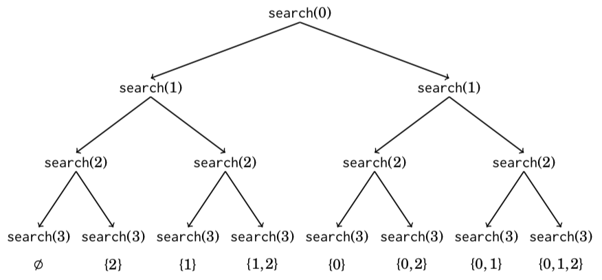
// 位运算枚举子集// Each subset of a set of n elements can be represented as a sequence of n bits,// which corresponds to an integer between 0...2n −1.// The ones in the bit sequence indicate which elements are included in the subset.//上面的程序,我们使用了一个vector来存储选了什么数字//这里,我们来学习一下位运算的枚举子集//这是一个拓展for (int b = 0; b < (1<<n); b++) {vector<int> subset;for (int i = 0; i < n; i++) {if (b&(1<<i)) subset.push_back(i);}}
例题,生成排列
For example, the permutations of {0,1,2} are (0,1,2), (0,2,1), (1,0,2), (1,2,0), (2,0,1) and (2,1,0).
// Each function call adds a new element to permutation.// The array chosen indicates which elements are already included in the permutation.// If the size of permutation equals the size of the set, a permutation has been generated.void search() {if (permutation.size() == n) {// process permutationreturn ;}for (int i = 0; i < n; i++) {if (chosen[i]) continue;chosen[i] = true;permutation.push_back(i);search();chosen[i] = false;permutation.pop_back();}}search(); //调用
// The C++ standard library contains the function next_permutation// that can be used for thisvector<int> permutation;for (int i = 0; i < n; i++) {permutation.push_back(i);}do {// process permutation} while (next_permutation(permutation.begin(),permutation.end()));
例题,递归实现指数型枚举
子集枚举
vector<int> chosen;void dfs(int x){if (x == n + 1) //也可以写x > n{for (int i = 0; i < chosen.size(); i++)printf("%d ", chosen[i]);puts("");return ;}//问:先不选x, 还是先选x。会影响我们的输出顺序//观察样例,我们先不选x//不选x,求解子问题dfs(x + 1);//选x,求解子问题chosen.push_back(x);dfs(x + 1);chosen.pop_back(); //回溯还原现场}
//位运算版本,这是进阶的void dfs(int u, int state){if (u == n){for (int i = 0; i < n; i++)if (state >> i & 1)cout << i + 1 << ' ';puts("");return ;}//求解子问题dfs(u + 1, state); //不选,state初始是0,等价于dfs(u + 1, state & (~(1 << u)));dfs(u + 1, state | 1 << u); //选}
例题,递归实现组合型枚举
在子集枚举的基础上,进行剪枝
vector<int> chosen;void dfs(int x){if (chosen.size() > m || chosen.size() + (n - x + 1) < m) return ;if (x == n + 1){//如何输出状态for (int i = 0; i < chosen.size(); i++)printf("%d ", chosen[i]);puts("");return ;}//选xchosen.push_back(x);dfs(x + 1);chosen.pop_back();//不选xdfs(x + 1);}
//递归实现,枚举的时候带着顺序void get_combination(int u, int last){if (u == m){for (int i = 0; i < m; i++) printf("%d ", chosen[i]);puts("");}for (int j = last + 1; j <= n; j++){chosen.push_back(j);get_combination(u + 1, j);chosen.pop_back();}}
//位运算版本,这是进阶的//state表示状态void dfs(int u, int sum, int state){if (sum > m || sum + n - u < m) return ;if (sum == m){for (int i = 0; i < n; i++)if (state >> i & 1)cout << i + 1 << ' ';puts("");return ;}dfs(u + 1, sum + 1, state | 1 << u);dfs(u + 1, sum , state );}
例题,递归实现排列型枚举
排列枚举
//用数组存方案//注意一下 0-index,如果是 1-index 呢?递归的边界是....什么?(提问)void dfs(int k){if (k == n){for (int i = 0; i < n; i++)cout << order[i] << ' ';puts("");}for (int i = 1; i <= n; i++){if (chosen[i]) continue;order[k] = i;chosen[i] = true;dfs(k + 1);chosen[i] = false;}}
// 用vector来存方案,用二进制数来记录状态vector<int> path;void dfs(int u, int state){if (u == n){vector<int>::iterator i;for (i = path.begin(); i < path.end(); i++)cout << *i << ' ';puts("");}for (int i = 0; i < n; i++)if (!(state >> i & 1)){path.push_back(i + 1); //用vector来记录方案dfs(u + 1, state | 1 << i);path.pop_back();}}
例题,NOIP 2012 普及组初赛试题,排列数
排列数 输入两个正整数n,m(1<n<20,1<m<n),在1~n中任取m个数,按字典序从小到大输出所有这样的排列。
//用贪心的方法,贪出来字典序#include <bits/stdc++.h>using namespace std;const int N = 110;int data[N];bool used[N];int n, m;int main(){cin >> n >> m;//第一种方案存了起来for (int i = 1; i <= m; i++){data[i] = i;used[i] = true;}bool flag = true;while (flag){//输出方案for (int i = 1; i <= m; i++) cout << data[i] << ' ';puts("");flag = false;for (int i = m; i >= 1; i--){used[data[i]] = false;for (int j = data[i] + 1; j <= n; j++){if (used[j] == false){data[i] = j;used[j] = true;flag = true;break;}}if (flag){for (int k = i + 1; k <= m; k++)for (int j = 1; j <= n; j++)if (used[j] == false){used[j] = true;data[k] = j;break;}break;}}}return 0;}
二分法
STL的使用(下标问题和避免SE)
//STLint pos = lower_bound(a, a + n, x) - a;int pos = upper_bound(a, a + n, x) - a;//lower_bound() 函数用于在指定区域内查找不小于目标值的第一个元素。也就是说,使用该函数在指定范围内查找某个目标值时,最终查找到的不一定是和目标值相等的元素,还可能是比目标值大的元素。//upper_bound() 函数的功能和 lower_bound() 函数不同,前者查找的是大于目标值的元素,而后者查找的不小于(大于或者等于)目标值的元素。
例题,和为给定数
//
binary search二分查找(有序序列中查找元素)
二分的基础用法是在单调序列或单调函数中进行查找。因此当问题的答案具有单调性时,就可以通过二分把求解转化为判定。其实,写二分的时候并不容易,写check函数的时候,有很多细节之处需要仔细考虑。
- 对于整数域上的二分,需要注意终止边界、左右区分取舍时的开闭请,避免漏掉进入死循环。
- 对于实数域上的二分,需要注意精度问题。
二分的实现模板有很多种,以下给出的模板是yxc的,非常好用。
//模板请记忆//整数二分bool check(int x) {/* ... */} // 检查x是否满足某种性质// 区间[l, r]被划分成[l, mid]和[mid + 1, r]时使用:int bsearch_1(int l, int r){while (l < r){int mid = l + r >> 1;if (check(mid)) r = mid; // check()判断mid是否满足性质else l = mid + 1;}return l;}// 区间[l, r]被划分成[l, mid - 1]和[mid, r]时使用:int bsearch_2(int l, int r){while (l < r){int mid = l + r + 1 >> 1;if (check(mid)) l = mid;else r = mid - 1;}return l;}//注意,分析题意,画数轴,看mid的右边是答案,还是mid的左边是答案
upd20211115,对于二分模板的认识,我现在认为不应该局限于模板本身,下面的代码更好去理解,也很专业。在初赛真题当中,有很多次二分,具体代码实现的环节,就有两种
while (l < r)while (l <= r)这两种在当时判断边界是用填空去写的,比较容易进坑,需要代数模拟。现在这两种写法一起组合,对二分的理解用会深入很多。边界确实是一个头疼的话题,很容错,然后,很难调。我现在更青睐后者
// 数的范围// https://www.acwing.com/problem/content/description/791/#include <bits/stdc++.h>using namespace std;const int N = 1e5 + 10;int n, q, a[N], k;int solve(int k){int l = 0, r = n - 1, best = -1;while (l <= r){int mid = (l + r) >> 1;if (a[mid] <= k){best = mid;l = mid + 1;}elser = mid - 1;}if (a[best] != k) return -1;return best;}int solve2(int k){int l = 0, r = n - 1, best = -1;while (l <= r){int mid = (l + r) >> 1;if (a[mid] >= k){best = mid;r = mid - 1;}elsel = mid + 1;}if (a[best] != k) return -1;return best;}int main(){cin >> n >> q;for (int i = 0; i < n; i++) scanf("%d", &a[i]);while (q--){scanf("%d", &k);int l = solve2(k);int r = solve(k);printf("%d %d\n", l, r);}return 0;}
//模板请记忆//浮点数二分,还有循环50次的写法bool check(double x) {/* ... */} // 检查x是否满足某种性质double bsearch_3(double l, double r){const double eps = 1e-6; // eps 表示精度,取决于题目对精度的要求while (r - l > eps){double mid = (l + r) / 2;if (check(mid)) r = mid;else l = mid;}return l;}double bsearch_4(double l, double r){int T = 50;while (T--){double mid = (l + r) / 2;if (check(mid)) r = mid;else l = mid;}return l;}
例题,和为给定数
//
例题,查找最接近的元素
//
二分答案(check函数的模拟)
一个宏观的最优化问题也可以抽象为函数,其“定义域”是该问题下的可行方案,对这些可行方案进行评估得到的数值构成函数的“值域”。假设评估得到的数值最高值是 s,对于大于 s 的都不合法,对于小于等于 s 的都是合法的,这样问题的值域就有一种特殊的单调性,在 s 的一侧合法,在 s 的另一侧不合法。借助二分,我们把求最优解的问题,转化为给定一个值 mid,判定是否存在一个可行方案评分达到 mid 的问题。
二分答案可以用来处理“最大的最小”或“最小的最大”问题。
常见问题:记录答案的二分写法,判断答案在哪边,check()函数经常写不准确的问题。
例题,网线主管
//
例题,月度开销
//
倍增法
快速幂(拓展移位运算,二进制的理解)
分治的方法
// 求:b^p// 思路:// 任意一个数p,可以表示成 p = 2 * p/2 + p%2// b^(2 * p/2 + p%2),就可以拆开后,递归调用f(p/2),递归终止边界是p == 0, return 1;
// 求2^b#include <iostream>using namespace std;int f(int b){if (b == 0) return 1;int t = f(b / 2);if (b & 1) return t * t * 2;else return t * t;}int main(){int a, b;cin >> b;cout << f(b) << '\n';return 0;}
// 求a^b#include <iostream>using namespace std;typedef long long ll;int f(int a, int b){if (b == 0) return 1;ll t = f(a, b / 2);if (b & 1) return t * t * a;else return t * t;}int main(){int a, b;cin >> a >> b;cout << f(a, b) << '\n';return 0;}
移位运算的方法

根据数学常识,每一个正整数可以唯一表示为若干个指数不重复的2的次幂的和。如果b在二进制下有k位,其中第i位的数字是 ,那么
,那么
于是:
因为 向上取整,所以上式乘积项的数量不多于k个,
又因为
所以,通过k次递推求出每个乘积项,当 时,把该乘积项累积到答案中。
b & 1 运算可以取出 b 在二进制表示下的最低位, 而 b >> 1 运算可以舍去最低位,在递推的过程中将二者结合,就可以遍历 b 在二进制表示下的所有数字  。时间复杂度是
  。
。
// 求 a^k mod p,时间复杂度 O(logk)// 模板请记忆// 写法1int qmi(int a, int k, int p){int res = 1;while (k) //当k不是0的时候{if (k & 1) res = (LL)res * a % p;k >>= 1;a = (LL)a * a % p;}return res;}// 写法2int power(int a, int b, int p){int ret = 1;for (; b; b >>= 1){if (b & 1) ret = 1ll * ret * a % p;a = 1ll * a * a % p;}return ret;}
例题,取余运算(mod)
输入b,p,k的值,求 b^p mod k 的值。其中b,p,k为长整型数。
例题,2011
通过测试发现,2011的n次方的结果,每500个数一循环。1次方、501次方、1001……结果一样。2次方,502次方,1002次方……结果一样。所以,尽管指数可能有200位,只需要考虑最后的3位指数就可以了。如果指数n不足3位,直接计算2011的n次方结果mod 10000就行了。
快速乘
快速乘法的说法来源于快速幂,因为两者的思想一致。快速幂是为了计算计算取模结果,的确是快的。而快速乘法主要是模数超过九次方时使用,因为两数相乘会longlong溢出,会比直接乘法慢,但是保证了正确性。所以说快速乘法并不快,想要比正常乘法快也是不现实的,快速乘法本来就是为了保证正确性而牺牲效率,自己实现了一遍乘法。要说快的话只能去和直接累加相比,就像快速幂比直接累乘取模快。
// 类似快速幂// 时间复杂度log(n)// 写法1int qmul(int a, int b, int p){int ret = 0;while (b){if (b & 1) ret = (ret + a) % p;b >>= 1;a = (a + a) % p;}return ret;}// 写法2typedef long long ll;ll qmul(ll a, ll b, ll p){ll ret = 0;for (; b; b >= 1){if (b & 1) ret = (ret + a) % p;a = a * 2 % p;}return ret;}
大纲要求
•【3】贪心法
•【3】递推法
•【4】递归法
•【4】二分法
•【4】倍增法

若有收获,就点个赞吧
0 人点赞
