在生物学中,注意力通常是由非自愿性提示以及自愿性提示主导的。非自愿性提示基于环境中对象的显眼性(人们倾向于注意到环境中显眼的东西);自愿性提示基于自身的意愿(你想喝咖啡,因此会注意到环境中的咖啡)
Queries,Keys,Values

了解了自愿性及非自愿性提示的概念后,再来看什么是QKV,Query对应自愿性提示,Keys实际上就是对应非自愿性提示,Value对应感官的输入。
注意力机制与普通全连接层以及池化层实际上是不同的,原因在于它们仅仅是Keys,但没有包含非自愿性提示(Query)。
Keys和Values是成对的。
Nadaraya-Watson Kernel Regression
这是一个1964年提出的经典算法,它可以诠释注意力机制在机器学习中是如何实现的。这一方法实际上就Attention Pooling的一种实现。
数据生成
考虑一个回归问题:给定一个键值对集,我们应该如何将这个函数f拟合出来?
现在我们人工基于规则构造一个数据集,其中为噪声项,它服从标准差为0.5,均值为0的正态分布
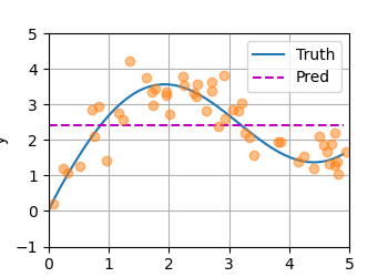
Average Pooling
先用一个非常弱智的函数看看拟合效果,就是将所有值求个平均:
Nonparametric Attention Pooling
平均池化忽略了输入Xi,那么Nadaraya和Watson想出了一个更好的拟合方式:
其中K是一个核函数,这里没必要管它。
回忆一下Attention中的QKV,我们可以将它表示成这样的形式:
事实上,这里的就是Query,而则是键值对。是注意力权重,所有键值对的注意力权重之和为1。
将K设为高斯核函数,可进行如下化简:
那么我们可以注意到,此处键与挨得越近,那么相应的就会得到更多的注意力。
总之,这是一种无参数注意力池化机制。效果好多了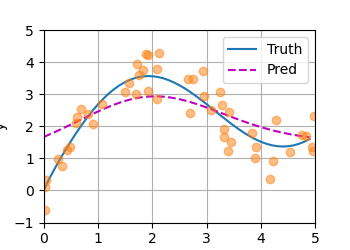
Parametric Attention Pooling
我们可以对回归函数再做一些改进,比如加一个参数:
Training
import torchfrom torch import nnfrom d2l import torch as d2ln_train = 50 # No. of training examplesx_train, _ = torch.sort(torch.rand(n_train) * 5) # Training inputsdef f(x):return 2 * torch.sin(x) + x ** 0.8y_train = f(x_train) + torch.normal(0.0, 0.5, (n_train,)) # Training outputsx_test = torch.arange(0, 5, 0.1) # Testing examplesy_truth = f(x_test) # Ground-truth outputs for the testing examplesn_test = len(x_test) # No. of testing examplesprint(n_test)def plot_kernel_reg(y_hat):d2l.plot(x_test, [y_truth, y_hat], 'x', 'y', legend=['Truth', 'Pred'],xlim=[0, 5], ylim=[-1, 5])d2l.plt.plot(x_train, y_train, 'o', alpha=0.5)d2l.plt.show()class NWKernelRegression(nn.Module):def __init__(self, **kwargs):super().__init__(**kwargs)self.w = nn.Parameter(torch.rand((1,), requires_grad=True))def forward(self, queries, keys, values):# Shape of the output `queries` and `attention_weights`:# (no. of queries, no. of key-value pairs)queries = queries.repeat_interleave(keys.shape[1]).reshape((-1, keys.shape[1]))self.attention_weights = nn.functional.softmax(-((queries - keys) * self.w)**2 / 2, dim=1)# Shape of `values`: (no. of queries, no. of key-value pairs)return torch.bmm(self.attention_weights.unsqueeze(1),values.unsqueeze(-1)).reshape(-1)# Shape of `X_tile`: (`n_train`, `n_train`), where each column contains the# same training inputsX_tile = x_train.repeat((n_train, 1))# Shape of `Y_tile`: (`n_train`, `n_train`), where each column contains the# same training outputsY_tile = y_train.repeat((n_train, 1))# Shape of `keys`: ('n_train', 'n_train' - 1)keys = X_tile[(1 - torch.eye(n_train)).type(torch.bool)].reshape((n_train, -1))# Shape of `values`: ('n_train', 'n_train' - 1)values = Y_tile[(1 - torch.eye(n_train)).type(torch.bool)].reshape((n_train, -1))net = NWKernelRegression()loss = nn.MSELoss(reduction='none')trainer = torch.optim.SGD(net.parameters(), lr=0.5)animator = d2l.Animator(xlabel='epoch', ylabel='loss', xlim=[1, 5])for epoch in range(5):trainer.zero_grad()# Note: L2 Loss = 1/2 * MSE Loss. PyTorch has MSE Loss which is slightly# different from MXNet's L2Loss by a factor of 2. Hence we halve the lossl = loss(net(x_train, keys, values), y_train) / 2l.sum().backward()trainer.step()print(f'epoch {epoch + 1}, loss {float(l.sum()):.6f}')animator.add(epoch + 1, float(l.sum()))# Shape of `keys`: (`n_test`, `n_train`), where each column contains the same# training inputs (i.e., same keys)keys = x_train.repeat((n_test, 1))# Shape of `value`: (`n_test`, `n_train`)values = y_train.repeat((n_test, 1))y_hat = net(x_test, keys, values).unsqueeze(1).detach()plot_kernel_reg(y_hat)
效果非常好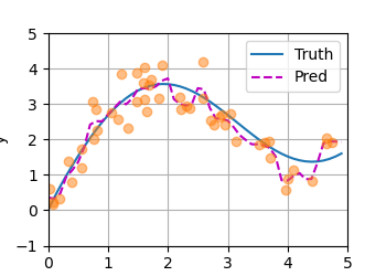

若有收获,就点个赞吧
0 人点赞
