重新索引
丢弃指定轴上的项
索引、选取和过滤
用loc和iloc进行选取
算术运算和数据对齐
在算数方法中填充值
DataFrame与Series之间的运算
函数的应用和映射
排序和排名
带有重复标签的轴索引

重新索引

pandas对象的一个重要方法是 reindex ，其作用是创建一个新对象，它的数据符合新的索引。看下面的例子

In [16]: obj = pd.Series([4.5, 2.2, 4.1, 1.4], index=['d', 'b', 'c', 'a'])
In [17]: obj
Out[17]:
d    4.5
b    2.2
c    4.1
a    1.4
dtype: float64
In [18]: obj2 = obj.reindex(['a', 'b', 'c', 'c'])
In [19]: obj2
Out[19]:
a    1.4
b    2.2
c    4.1
c    4.1
dtype: float64

对于时间序列这样的有序数据，重新索引时可能需要做一些插值处理。 method 选项即可达到此目的。例如，使用 ffukk 可以实现前向值填充

In [20]: obj3 = pd.Series(['blue', 'purple', 'yellow'], index=[0,2,4])
In [21]: obj3
Out[21]:
0      blue
2    purple
4    yellow
dtype: object
In [22]: obj3.reindex(range(6), method='ffill')
Out[22]:
0      blue
1      blue
2    purple
3    purple
4    yellow
5    yellow
dtype: object

借助DataFrame， reindex 可以修改（行）索引和列。只传递一个序列时，会重新索引结果的行

In [23]: frame = pd.DataFrame(np.arange(9).reshape((3,3)),
    ...:                      index=['a', 'c', 'd'],
    ...:                      columns=['Ohio', 'Texas', 'California'])
In [24]: frame
Out[24]:
   Ohio  Texas  California
a     0      1           2
c     3      4           5
d     6      7           8
In [25]: frame2 = frame.reindex(['a', 'b', 'c', 'd'])
In [26]: frame2
Out[26]:
   Ohio  Texas  California
a   0.0    1.0         2.0
b   NaN    NaN         NaN
c   3.0    4.0         5.0
d   6.0    7.0         8.0

列可以用 columns 关键字重新索引

In [27]: states = ['Texas', 'Utah', 'California']
In [28]: frame.reindex(columns=states)
Out[28]:
   Texas  Utah  California
a      1   NaN           2
c      4   NaN           5
d      7   NaN           8

reindex 函数的参数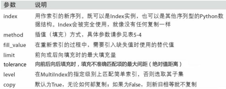

丢弃指定轴上的项

丢弃某条轴上的一个或多个项很简单，只要有一个索引数组或列表即可。由于需要执行一些数据整理和集合逻辑，所以 drop 方法返回的是一个在指定轴上删除了指定值的新对象

In [3]: obj = pd.Series(np.arange(5.), index=['a', 'b', 'c', 'd', 'e'])
In [4]: obj
Out[4]:
a    0.0
b    1.0
c    2.0
d    3.0
e    4.0
dtype: float64
In [5]: new_obj = obj.drop('c')
In [6]: new_obj
Out[6]:
a    0.0
b    1.0
d    3.0
e    4.0
dtype: float64

对于DataFrame，可以删除任意轴上的索引值。为了演示，先新建一个DataFrame例子

In [7]: data = pd.DataFrame(np.arange(16).reshape((4,4)),
   ...:                     index=['Ohio', 'Colorado', 'Utah', 'New York'],
   ...:                     columns=['one', 'two', 'three', 'four'])
In [8]: data
Out[8]:
          one  two  three  four
Ohio        0    1      2     3
Colorado    4    5      6     7
Utah        8    9     10    11
New York   12   13     14    15

用标签序列调用 drop 会从行标签（axis=0）删除值

In [9]: data.drop(['Colorado', 'Ohio'])
Out[9]:
          one  two  three  four
Utah        8    9     10    11
New York   12   13     14    15

通过传递axis=1或axis=’columns’可以删除列的值

In [10]: data.drop('two', axis=1)
Out[10]:
          one  three  four
Ohio        0      2     3
Colorado    4      6     7
Utah        8     10    11
New York   12     14    15
In [11]: data.drop(['two', 'four'], axis='columns')
Out[11]:
          one  three
Ohio        0      2
Colorado    4      6
Utah        8     10
New York   12     14

许多函数，如drop ，会修改Series或DataFrame的大小或形状，可以就地修改对象，不会返回新的对象

In [12]: obj.drop('c', inplace=True)
In [13]: obj
Out[13]:
a    0.0
b    1.0
d    3.0
e    4.0
dtype: float64

小心使用inplace，它会销毁所有被删除的数据

索引、选取和过滤

Series索引（ obj[...] ）的工作方式类似于NumPy数组的索引，只不过Series的索引值不只是整数。下面是几个例子

In [14]: obj = pd.Series(np.arange(4.), index=['a', 'b', 'c', 'd'])
In [15]: obj
Out[15]:
a    0.0
b    1.0
c    2.0
d    3.0
dtype: float64
In [16]: obj['b']
Out[16]: 1.0
In [17]: obj[1]
Out[17]: 1.0
In [18]: obj[2:4]
Out[18]:
c    2.0
d    3.0
dtype: float64
In [19]: obj[['b', 'a', 'd']]
Out[19]:
b    1.0
a    0.0
d    3.0
dtype: float64
In [20]: obj[[1,3]]
Out[20]:
b    1.0
d    3.0
dtype: float64
In [21]: obj[obj < 2]
Out[21]:
a    0.0
b    1.0
dtype: float64

利用标签的切片运算与普通的Python切片运算不同，其末端是包含的

In [22]: obj['b':'c']
Out[22]:
b    1.0
c    2.0
dtype: float64

用切片可以对Series的相应部分进行设置

In [23]: obj['b':'c'] = 5
In [24]: obj
Out[24]:
a    0.0
b    5.0
c    5.0
d    3.0
dtype: float64

用一个值或序列对DataFrame进行索引其实就是获取一个或多个列

In [25]: data = pd.DataFrame(np.arange(16).reshape((4,4)),
    ...:                     index=['Ohio', 'Colorado', 'Utah', 'New York'],
    ...:                     columns=['one', 'two', 'three', 'four'])
In [26]: data
Out[26]:
          one  two  three  four
Ohio        0    1      2     3
Colorado    4    5      6     7
Utah        8    9     10    11
New York   12   13     14    15
In [27]: data['two']
Out[27]:
Ohio         1
Colorado     5
Utah         9
New York    13
Name: two, dtype: int32
In [28]: data[['three', 'one']]
Out[28]:
          three  one
Ohio          2    0
Colorado      6    4
Utah         10    8
New York     14   12

这种索引方式有几个特殊的情况。首先通过切片或布尔型数组选取数据

In [29]: data[:2]
Out[29]:
          one  two  three  four
Ohio        0    1      2     3
Colorado    4    5      6     7
In [30]: data[data['three'] > 5]
Out[30]:
          one  two  three  four
Colorado    4    5      6     7
Utah        8    9     10    11
New York   12   13     14    15

选取行的语法 data[:2] 十分方便。向 [] 传递单一的元素或列表，就可选择列
另一种用法是通过布尔型DataFrame（比如下面这个由标量比较运算得出的）进行索引

In [32]: data < 5
Out[32]:
            one    two  three   four
Ohio       True   True   True   True
Colorado   True  False  False  False
Utah      False  False  False  False
New York  False  False  False  False
In [33]: data[data < 5] = 0
In [34]: data
Out[34]:
          one  two  three  four
Ohio        0    0      0     0
Colorado    0    5      6     7
Utah        8    9     10    11
New York   12   13     14    15

这使得DataFrame的语法与NumPy二维数组的语法很像

用loc和iloc进行选取

对于DataFrame的行的标签索引，我引入了特殊的标签运算符 loc 和iloc 。它们可以让你用类似NumPy的标记，使用轴标签（ loc ）或整数索引（ iloc ），从DataFrame选择行和列的子集
作为一个初步示例，让我们通过标签选择一行和多列

In [36]: data.loc['Colorado', ['two', 'three']]
Out[36]:
two      5
three    6
Name: Colorado, dtype: int32

然后用 iloc 和整数进行选取

In [4]: data.iloc[2, [3, 0, 1]]
Out[4]:
four    11
one      8
two      9
Name: Utah, dtype: int32
In [5]: data.iloc[2]
Out[5]:
one       8
two       9
three    10
four     11
Name: Utah, dtype: int32
In [6]: data.iloc[[1,2], [3,0,1]]
Out[6]:
          four  one  two
Colorado     7    4    5
Utah        11    8    9

这两个索引函数也适用于一个标签或多个标签的切片

这有点类似SQL中 where ```python In [7]: data.loc[‘Utah’, ‘two’] Out[7]: 9

In [8]: data.iloc[:, :3][data.three > 5] Out[8]: one two three Colorado 4 5 6 Utah 8 9 10 New York 12 13 14

下表展示了对**DataFrame**进行选取和重新组合的多个方法<br />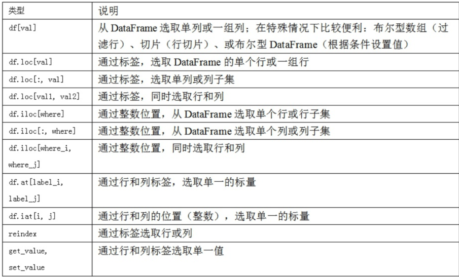![image.png](https://cdn.nlark.com/yuque/0/2020/png/805730/1590826395826-6e460aa7-e4ed-408e-a91f-0e84cde2901a.png#align=left&display=inline&height=410&margin=%5Bobject%20Object%5D&name=image.png&originHeight=547&originWidth=905&size=405861&status=done&style=none&width=679)
<a name="XBuun"></a>
# 整数索引
**pandas**可以勉强进行整数索引，但是会导致小bug。我们有包含0,1,2的索引，但是引入用户想要的东西（基于标签或位置的索引）很难。下面的代码会出错。因为玩意-1也是索引值呢？
```python
ser = pd.Series(np.arange(3.))
ser
ser[-1]

另外，对于非整数索引，不会产生歧义

In [11]: ser2 = pd.Series(np.arange(3.), index=['a', 'b', 'c'])
In [12]: ser2[-1]
Out[12]: 2.0

为了进行统一，如果轴索引含有整数，数据选取总会使用标签。为了更准确，请使用 **loc** （标签）或 iloc （整数）

算术运算和数据对齐

pandas最重要的一个功能是，它可以对不同索引的对象进行算术运算。在将对象相加时，如果存在不同的索引对，则结果的索引就是该索引对的并集。对于有数据库经验的用户，这就像在索引标签上进行自动外连接。看一个简单的例子

In [13]: s1 = pd.Series([7.3, -2.5, 3.4, 2.1], index=['a', 'c', 'd', 'e'])
In [14]: s2 = pd.Series([-2.1, 2.2, 1.3, 4.5, 5.3], index=['a', 'c', 'e', 'f', 'g'])
In [15]: s1
Out[15]:
a    7.3
c   -2.5
d    3.4
e    2.1
dtype: float64
In [16]: s2
Out[16]:
a   -2.1
c    2.2
e    1.3
f    4.5
g    5.3
dtype: float64

现在让它们做加法

In [17]: s1 + s2
Out[17]:
a    5.2
c   -0.3
d    NaN
e    3.4
f    NaN
g    NaN
dtype: float64

自动的数据对齐操作在不重叠的索引处引入了NA值。缺失值会在算术运算过程中传播
对于DataFrame，对齐操作会同时发生在行和列上

In [18]: df1 = pd.DataFrame(np.arange(9.).reshape((3,3)), columns=list('bcd'),
    ...:                    index=['Ohio', 'Texas', 'Colorado'])
In [19]: df2 = pd.DataFrame(np.arange(12.).reshape((4,3)), columns=list('bde'),
    ...:                    index=['Utah', 'Ohio', 'Texas', 'Oregon'])
In [20]: df1
Out[20]:
            b    c    d
Ohio      0.0  1.0  2.0
Texas     3.0  4.0  5.0
Colorado  6.0  7.0  8.0
In [21]: df2
Out[21]:
          b     d     e
Utah    0.0   1.0   2.0
Ohio    3.0   4.0   5.0
Texas   6.0   7.0   8.0
Oregon  9.0  10.0  11.0

把它们相加后将会返回一个新的DataFrame，其索引和列为原来那两个DataFrame的并集

In [22]: df1 + df2
Out[22]:
            b   c     d   e
Colorado  NaN NaN   NaN NaN
Ohio      3.0 NaN   6.0 NaN
Oregon    NaN NaN   NaN NaN
Texas     9.0 NaN  12.0 NaN
Utah      NaN NaN   NaN NaN

因为’c‘和’e‘列均不在两个DataFrame对象中，在结果中以缺省值呈现。行也是同样
如果DataFrame对象相加，没有共用的列或行标签，结果都会是空

In [24]: df1 = pd.DataFrame({'A':[1,2]})
In [25]: df2 = pd.DataFrame({'B': [3,4]})
In [26]: df1
Out[26]:
   A
0  1
1  2
In [27]: df2
Out[27]:
   B
0  3
1  4
In [28]: df1 - df2
Out[28]:
    A   B
0 NaN NaN
1 NaN NaN

在算数方法中填充值

在对不同索引的对象进行算术运算时，你可能希望当一个对象中某个轴标签在另一个对象中找不到时填充一个特殊值（比如0）

In [29]: df1 = pd.DataFrame(np.arange(12.).reshape((3,4)), columns=list('abcd'))
In [30]: df2 = pd.DataFrame(np.arange(20.).reshape((4,5)), columns=list('abcde'))
In [31]: df2.loc[1, 'b'] = np.nan
In [32]: df1
Out[32]:
     a    b     c     d
0  0.0  1.0   2.0   3.0
1  4.0  5.0   6.0   7.0
2  8.0  9.0  10.0  11.0
In [33]: df2
Out[33]:
      a     b     c     d     e
0   0.0   1.0   2.0   3.0   4.0
1   5.0   NaN   7.0   8.0   9.0
2  10.0  11.0  12.0  13.0  14.0
3  15.0  16.0  17.0  18.0  19.0

将它们相加时，没有重叠的位置就会产生NA值

In [34]: df1 + df2
Out[34]:
      a     b     c     d   e
0   0.0   2.0   4.0   6.0 NaN
1   9.0   NaN  13.0  15.0 NaN
2  18.0  20.0  22.0  24.0 NaN
3   NaN   NaN   NaN   NaN NaN

使用 df1 的 add 方法，传入 df2 以及一个fill_value 参数

注意这个方法的结果和上例中直接使用加法运算符的差别

In [35]: df1.add(df2, fill_value=0)
Out[35]:
    a     b     c     d     e
0   0.0   2.0   4.0   6.0   4.0
1   9.0   5.0  13.0  15.0   9.0
2  18.0  20.0  22.0  24.0  14.0
3  15.0  16.0  17.0  18.0  19.0

```python In [36]: 1 / df1 Out[36]:

 a         b         c         d

0 inf 1.000000 0.500000 0.333333 1 0.250 0.200000 0.166667 0.142857 2 0.125 0.111111 0.100000 0.090909

In [37]: df1.rdiv(1) Out[37]: a b c d 0 inf 1.000000 0.500000 0.333333 1 0.250 0.200000 0.166667 0.142857 2 0.125 0.111111 0.100000 0.090909

下表列出了**Series**和**DataFrame**的算数方法。它们每个都有一个副本，以字母r开头，它会翻转参数。因此上面两个语句是等价的<br />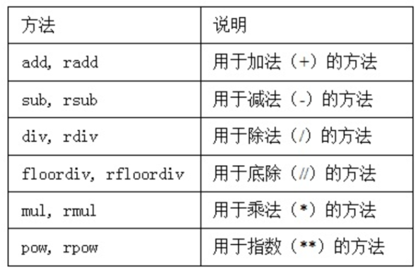![image.png](https://cdn.nlark.com/yuque/0/2020/png/805730/1590828062056-7ce5fce4-10d0-4cbd-9d64-97496c4b15da.png#align=left&display=inline&height=288&margin=%5Bobject%20Object%5D&name=image.png&originHeight=384&originWidth=592&size=101952&status=done&style=none&width=444)<br />与此类似，在对**Series**或**DataFrame**重新索引时，也可以指定一个填充值
```python
In [38]: df1.reindex(columns=df2.columns, fill_value=0)
Out[38]:
     a    b     c     d  e
0  0.0  1.0   2.0   3.0  0
1  4.0  5.0   6.0   7.0  0
2  8.0  9.0  10.0  11.0  0

DataFrame与Series之间的运算

跟不同维度的NumPy数组一样，DataFrame和Series之间算术运算也是有明确规定的。先看一个启发性的例子

In [44]: arr = np.arange(12.).reshape((3,4))
In [45]: arr[0]
Out[45]: array([0., 1., 2., 3.])
In [46]: arr - arr[0]
Out[46]:
array([[0., 0., 0., 0.],
       [4., 4., 4., 4.],
       [8., 8., 8., 8.]])

当我们从 arr 减去 arr[0] ，每一行都会执行这个操作。这就叫做广播（broadcasting）DataFrame和Series之间的运算也差不多

In [49]: frame = pd.DataFrame(np.arange(12.).reshape((4,-1)),
    ...:                      columns=list('bde'),
    ...:                      index=['Utah', 'Ohio', 'Texas', 'Oregon'])
In [50]: series = frame.iloc[0]
In [51]: frame
Out[51]:
          b     d     e
Utah    0.0   1.0   2.0
Ohio    3.0   4.0   5.0
Texas   6.0   7.0   8.0
Oregon  9.0  10.0  11.0
In [52]: series
Out[52]:
b    0.0
d    1.0
e    2.0
Name: Utah, dtype: float64

默认情况下，DataFrame和Series之间的算术运算会将Series的索引匹配到DataFrame的列，然后沿着行一直向下广播

In [53]: frame - series
Out[53]:
          b    d    e
Utah    0.0  0.0  0.0
Ohio    3.0  3.0  3.0
Texas   6.0  6.0  6.0
Oregon  9.0  9.0  9.0

如果某个索引值在DataFrame的列或Series的索引中找不到，则参与运算的两个对象就会被重新索引以形成并集

从上例中，Series是DataFrame中的一行，所以Series中的 index 是DataFrame中的 column
下例中，只有’b‘和’e‘匹配到了索引，而这两列对应的分别是0和1，所以 frame 中的列’b’和’e’分别都通过广播，加上了0和1 ```python In [54]: series2 = pd.Series(range(3), index=[‘b’, ‘e’, ‘f’])

In [55]: frame + series2 Out[55]: b d e f Utah 0.0 NaN 3.0 NaN Ohio 3.0 NaN 6.0 NaN Texas 6.0 NaN 9.0 NaN Oregon 9.0 NaN 12.0 NaN

如果你希望匹配行且在列上广播， 则必须使用算术运算方法
```python
In [56]: series3 = frame['d']
In [57]: frame
Out[57]:
          b     d     e
Utah    0.0   1.0   2.0
Ohio    3.0   4.0   5.0
Texas   6.0   7.0   8.0
Oregon  9.0  10.0  11.0
In [58]: series3
Out[58]:
Utah       1.0
Ohio       4.0
Texas      7.0
Oregon    10.0
Name: d, dtype: float64
In [59]: frame.sub(series3, axis='index')
Out[59]:
          b    d    e
Utah   -1.0  0.0  1.0
Ohio   -1.0  0.0  1.0
Texas  -1.0  0.0  1.0
Oregon -1.0  0.0  1.0

传入的轴号就是希望匹配的轴。在本例中，我们的目的是匹配DataFrame的行索引（ axis='index' oraxis=0 ）并进行广播

函数的应用和映射

NumPy的ufuncs（元素级数组方法）也可用于操作pandas对象

In [4]: frame = pd.DataFrame(np.random.randn(4,3), columns=list('bde'),
   ...:                      index=['Utah', 'Ohio', 'Texas', 'Oregon'])
In [5]: frame
Out[5]:
               b         d         e
Utah    0.298742 -0.546586 -0.689643
Ohio   -0.592324  1.528673 -0.450995
Texas   1.112818  0.870985  0.422259
Oregon  1.096166 -1.183010  0.905282
In [6]: np.abs(frame)
Out[6]:
               b         d         e
Utah    0.298742  0.546586  0.689643
Ohio    0.592324  1.528673  0.450995
Texas   1.112818  0.870985  0.422259
Oregon  1.096166  1.183010  0.905282

另一个常见的操作是，将函数应用到由各列或行所形成的一维数组上。DataFrame的 apply 方法即可实现此功能

In [7]: f = lambda x: x.max() - x.min()
In [8]: frame.apply(f)
Out[8]:
b    1.705142
d    2.711683
e    1.594925
dtype: float64

这里的函数 f ，计算了一个Series的最大值和最小值的差，在frame 的每列都执行了一次。结果是一个Series，使用 frame 的列作为索引

如果传递 axis='columns' 到 apply ，这个函数会在每行执行

In [10]: frame.apply(f, axis='columns')
Out[10]:
Utah      0.988385
Ohio      2.120997
Texas     0.690559
Oregon    2.279176
dtype: float64

许多最为常见的数组统计功能都被实现成DataFrame的方法（如 sum 和mean ），因此无需使用 apply 方法
传递到apply 的函数不是必须返回一个标量，还可以返回由多个值组成的Series

In [11]: def f(x):
    ...:     return pd.Series([x.min(), x.max()], index=['min', 'max'])
    ...:
In [12]: frame.apply(f)
Out[12]:
            b         d         e
min -0.592324 -1.183010 -0.689643
max  1.112818  1.528673  0.905282

元素级的Python函数也是可以用的。假如你想得到frame 中各个浮点值的格式化字符串，使用applymap 即可

In [13]: format = lambda x : '%.2f' % x
In [14]: frame.applymap(format)
Out[14]:
            b      d      e
Utah     0.30  -0.55  -0.69
Ohio    -0.59   1.53  -0.45
Texas    1.11   0.87   0.42
Oregon   1.10  -1.18   0.91

之所以叫做applymap ，是因为Series有一个用于应用元素级函数的map 方法

In [15]: frame['e'].map(format)
Out[15]:
Utah      -0.69
Ohio      -0.45
Texas      0.42
Oregon     0.91
Name: e, dtype: object

排序和排名

根据条件对数据集排序（sorting）也是一种重要的内置运算。要对行或列索引进行排序（按字典顺序），可使用sort_index 方法，它将返回一个已排序的新对象

In [16]: obj = pd.Series(range(4), index=['d', 'a', 'b', 'c'])
In [17]: obj.sort_index()
Out[17]:
a    1
b    2
c    3
d    0
dtype: int64

对于DataFrame，则可以根据任意一个轴上的索引进行排序

In [18]: frame = pd.DataFrame(np.arange(8.).reshape((2,4)),
    ...:                      index=['three', 'one'],
    ...:                      columns=['d', 'a', 'b', 'c'])
In [19]: frame.sort_index()
Out[19]:
         d    a    b    c
one    4.0  5.0  6.0  7.0
three  0.0  1.0  2.0  3.0
In [20]: frame.sort_index(axis=1)
Out[20]:
         a    b    c    d
three  1.0  2.0  3.0  0.0
one    5.0  6.0  7.0  4.0

数据默认是按升序排序的，但也可以降序排序

In [21]: frame.sort_index(axis=1, ascending=False)
Out[21]:
         d    c    b    a
three  0.0  3.0  2.0  1.0
one    4.0  7.0  6.0  5.0

若要按值对Series进行排序，可使用其sort_values 方法

In [23]: obj.sort_values()
Out[23]:
2   -3
3    2
0    4
1    7
dtype: int64

在排序时，任何缺失值默认都会被放到Series的末尾

In [25]: obj.sort_values()
Out[25]:
4   -3.0
5    2.0
0    4.0
2    7.0
1    NaN
3    NaN
dtype: float64

当排序一个DataFrame时，你可能希望根据一个或多个列中的值进行排序。将一个或多个列的名字传递给sort_values 的 by 选项即可达到该目的

In [29]: frame.sort_values(by='b')
Out[29]:
   b  a
2 -3  0
3  2  1
0  4  0
1  7  1

要根据多个列进行排序，传入名称的列表即可

In [30]: frame.sort_values(by=['a', 'b'])
Out[30]:
   b  a
2 -3  0
0  4  0
3  2  1
1  7  1

排名会从1开始一直到数组中有效数据的数量。接下来介绍Series和DataFrame的 rank 方法。默认情况下， rank 是通过“为各组分配一个平均排名”的方式破坏平级关系的

In [32]: obj = pd.Series([7, -5, 7, 4 ,2, 0, 4])
In [33]: obj.rank()
Out[33]:
0    6.5
1    1.0
2    6.5
3    4.5
4    3.0
5    2.0
6    4.5
dtype: float64

也可以根据值在原数据中出现的顺序给出排名

In [34]: obj.rank(method='first')
Out[34]:
0    6.0
1    1.0
2    7.0
3    4.0
4    3.0
5    2.0
6    5.0
dtype: float64

这里，条目0和2没有使用平均排名6.5，它们被设成了6和7，因为数据中标签0位于标签2的前面。
你也可以按降序进行排名

In [35]: obj.rank(ascending=False, method='max')
Out[35]:
0    2.0
1    7.0
2    2.0
3    4.0
4    5.0
5    6.0
6    4.0
dtype: float64

下表列出了所有用于破坏平级关系的method 选项。DataFrame可以在行或列上计算排名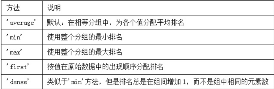

In [36]: frame = pd.DataFrame({'b': [4.3, 7, -3 ,2], 'a': [0, 1, 0, 1],
    ...:                       'c': [-2, 5, 8, -2.5]})
In [37]: frame
Out[37]:
     b  a    c
0  4.3  0 -2.0
1  7.0  1  5.0
2 -3.0  0  8.0
3  2.0  1 -2.5
In [38]: frame.rank(axis='columns')
Out[38]:
     b    a    c
0  3.0  2.0  1.0
1  3.0  1.0  2.0
2  1.0  2.0  3.0
3  3.0  2.0  1.0

带有重复标签的轴索引

虽然许多pandas函数（如reindex ）都要求标签唯一，但这并不是强制性的。我们来看看下面这个简单的带有重复索引值的Series

In [39]: obj = pd.Series(range(5), index=['a', 'a', 'b', 'b', 'c'])
In [40]: obj
Out[40]:
a    0
a    1
b    2
b    3
c    4
dtype: int64

索引的in_unique 属性可以告诉你它的值是否是唯一的

In [42]: obj.index.is_unique
Out[42]: False

对于带有重复值的索引，数据选取的行为将会有些不同。如果某个索引对应多个值，则返回一个Series；而对应单个值的，则返回一个标量值

In [43]: obj['a']
Out[43]:
a    0
a    1
dtype: int64
In [44]: obj['c']
Out[44]: 4

这样会使代码变复杂，因为索引的输出类型会根据标签是否有重复发生变化
对DataFrame的行进行索引时也是如此

In [45]: df = pd.DataFrame(np.random.randn(4, 3), index=['a', 'a', 'b', 'b'])
In [46]: df
Out[46]:
          0         1         2
a  0.598633  0.509012 -0.319608
a  0.545685 -0.724553 -0.731425
b -0.971970  0.674816  0.304169
b -0.190280 -2.692565  1.386602
In [47]: df.loc['b']
Out[47]:
         0         1         2
b -0.97197  0.674816  0.304169
b -0.19028 -2.692565  1.386602

Programming Language

【Pandas入门】基本功能