1 入门 Tips

1.1 Import Matplotlib

就像我们使用 np 和 pd 来代表 numpy 和 pandas 一样，我们对 matplotlib 也有以下约定俗成的命名方式：

import matplotlib as mpl
import matplotlib.pyplot as plt

plt 是本章节最常用的接口。

1.2 设置样式 (Setting Styles)

我们使用 plt.style 来选择合适的图表样式。下面我们设置了 classic 样式：

plt.style.use('classic')

1.3 show() or No show() ? 如何展示画出来的图表？

我们知道，Matplotlib 画出来的图表取决于你前面所编写的代码的。大概有 3 种使用 Matplotlib 的方法：

• 在脚本文件中使用
• 在 IPython terminal 中使用
• 在 IPython notebook 中使用

1.3.1 在脚本文件中 plot

如果在脚本文件中使用 Matplotlib，那么 plt.show() 是必要的。 plt.show() 启动一个事件循环（不断监听事件并响应，比如鼠标拖动等），并且打开一个或多个交互式的窗口来展示图表。

假设我们现在有一个名叫 myplot.py 的文件，并且存有以下代码：

# ------- file: myplot.py -------
import matplotlib as mpl
import matplotlib.pyplot as plt
x= np.linspace(0, 10, 100)
plt.plot(x, np.sin(x))
plt.plot(x, np.cos(x))
plt.show()

然后就可以以各种方式（命令行或 IDE 等）运行这个 Python 脚本，随后就会看到一个新的窗口，窗口里有你刚刚画的图。

需要注意的一点是： plt.show() 在一个 Python 会话 ( session ) 中只能使用一次，并且我们经常把它放在脚本代码的最后。多个 plt.show() 。。。就。。。嗯。。。

1.3.2 在 IPython shell 中 plot

IPython 专门为 Matplotlib 设置了一个模式，使用 %matplotlib 魔术指令来开启：

In [1]: %matplotlib
Using matplotlib backend: Qt5Agg
In [2]: import matplotlib.pyplot as plt

这个时候，每当你使用 plt.plot() 都会立即创建一个新的窗口来展示你画出来的图表，而不是等到 show()的时候才会统一展示。

1.3.3 在 IPython notebook 中 plot

在 IPython notebook 中也是使用 %matplotlib 命令来交互式地使用 Matplotlib 的。但是，在 IPython notebook 中，还有两种额外的选项可以帮助你将图表嵌入到 notebook 中：

• %matplotlib notebook —- 在 notebook 中嵌入动态交互式的图表
• %matplotlib inline—- 在 notebook 中嵌入静态的图表

一般我们都使用 %matplotlib inline 。在 notebook 的一个 cell 中运行如下代码：

import numpy as np
x = np.linspace(0, 10, 100)
fig = plt.figure()
plt.plot(x, np.sin(x), '-')
plt.plot(x, np.cos(x), '--');

效果如下：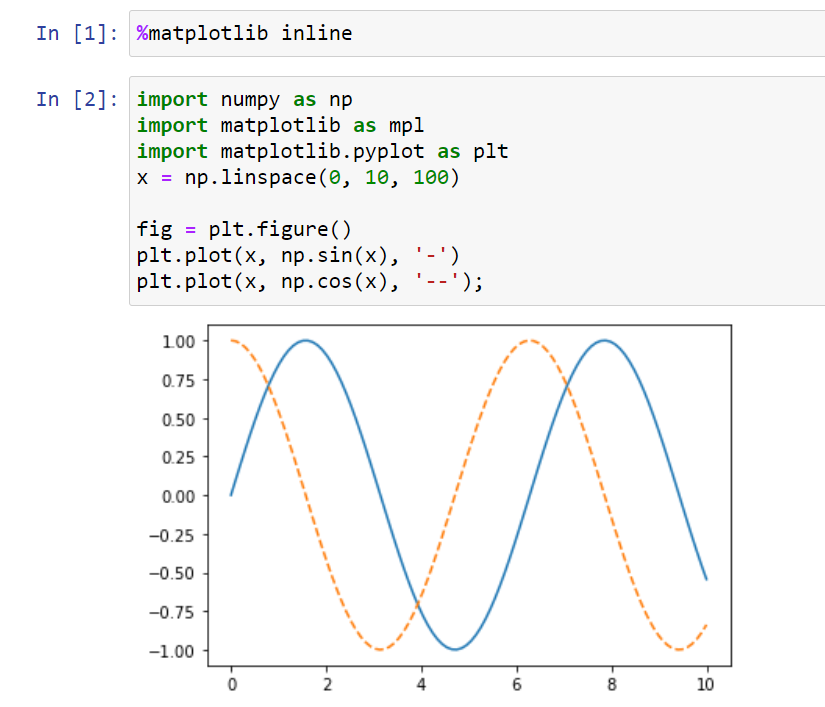

1.4 保存图表 savefig()

使用 savefig() 命令可以将刚才画出来的图表保存到本地：

fig.savefig('my_figure.png')

然后使用 IPython 的 Image 对象来展示刚才保存的图片：

from IPython.display import Image
Image('my_figure.png')

效果如下：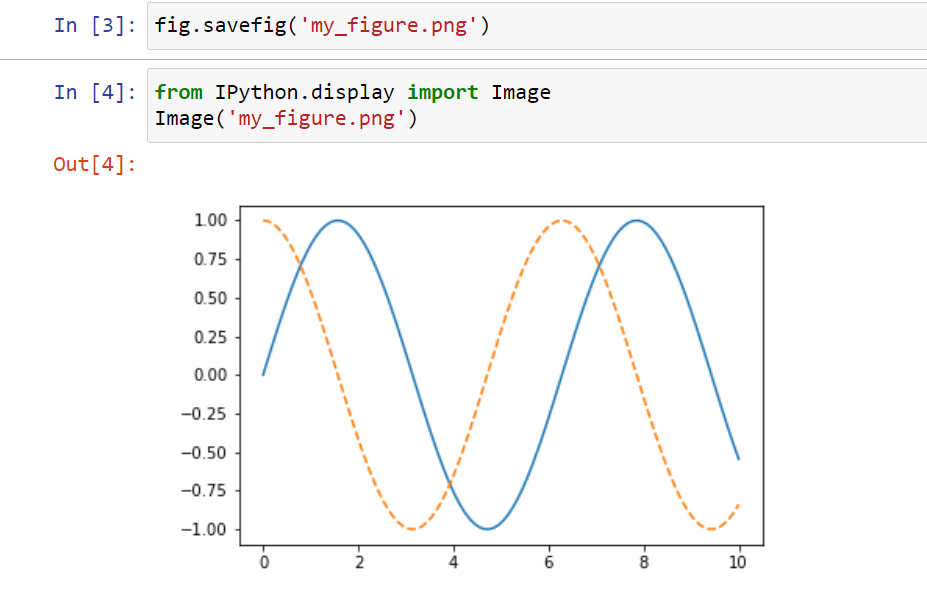

在 savefig() 中你可以选择多种保存图片的格式（设定文件扩展名）。可以使用 figure 的 canvas 对象来获取支持保存的图片格式：

In [5]: fig.canvas.get_supported_filetypes()
Out[5]: {'eps': 'Encapsulated Postscript',
         'jpg': 'Joint Photographic Experts Group',
         'jpeg': 'Joint Photographic Experts Group',
         'pdf': 'Portable Document Format',
         'pgf': 'PGF code for LaTeX',
         'png': 'Portable Network Graphics',
         'ps': 'Postscript',
         'raw': 'Raw RGBA bitmap',
         'rgba': 'Raw RGBA bitmap',
         'svg': 'Scalable Vector Graphics',
         'svgz': 'Scalable Vector Graphics',
         'tif': 'Tagged Image File Format',
         'tiff': 'Tagged Image File Format'}

2 mpl 两种风格的接口

2.1 MATLAB 风格

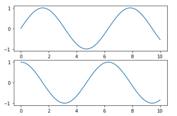
plt.figure()  # create a plot figure
# create the first of two panels and set current axis
plt.subplot(2, 1, 1) # (rows, columns, panel number)
plt.plot(x, np.sin(x))
# create the second panel and set current axis
plt.subplot(2, 1, 2)
plt.plot(x, np.cos(x));

注意：这种接口是有状态的 ( stateful )： plt 使用过的指令都会体现在当前 ( current ) 的表格和坐标轴上。
可以使用 plt.gcf() ( get current figure ) 以及 plt.gca() ( get current axes ) 来获取。

虽然这种有状态的接口运行速度快并且非常适合简单图表的绘制，但也会导致一些问题：假如我们已经执行到 plt.subplot(2, 1, 2) 开始在第二个子图中画东西，那么如何回到第一个子图添加一点别的东西呢？这可以实现，但是比较麻烦，所以有下面面向对象风格的接口来解决问题！

2.2 面向对象风格

面向对象风格的接口一般用于比较复杂的绘图场景，这可以让你更加灵活的控制你的图表。
在面向对象风格的接口中，绘图函数都以方法 ( methods ) 的形式由 Figure 和 Axes 对象提供。

# First create a grid of plots
# ax will be an array of two Axes objects
fig, ax = plt.subplots(2)
# Call plot() method on the appropriate object
ax[0].plot(x, np.sin(x))
ax[1].plot(x, np.cos(x));

绘图的结果同样如上。