参考https://www.cnblogs.com/think90/p/7133753.html
- 组内平方误差和——拐点图(肘部法则SSE)
- 轮廓系数
1. 组内平方误差和——拐点图(肘部法则SSE)
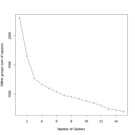
随着聚类数目增多,每一个类别中数量越来越少,距离越来越近,因此WSS值肯定是随着聚类数目增多而减少的,所以关注的是斜率的变化,但WWS减少得很缓慢时,就认为进一步增大聚类数效果也并不能增强,存在得这个“肘点”就是最佳聚类数目,从一类到三类下降得很快,之后下降得很慢,所以最佳聚类个数选为3。
2. 轮廓系数
轮廓系数是类的密集与分散程度的评价指标。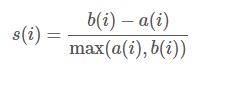
a(i)是测量组内的样本i在到其它点的平均距离,b(i)是测量组间的样本i到最近不同类别中样本的平均距离,s(i)范围从-1到1,值越大说明组内吻合越高,组间距离越远——也就是说,轮廓系数值越大,聚类效果越好。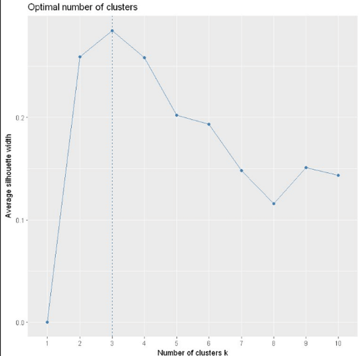
3. 实现
参考 https://www.cnblogs.com/feffery/p/12325741.html
我是直接拷贝https://github.com/arvkevi/kneed/blob/master/kneed/knee_locator.py 的实现,这就不用安装kneed模块了。
(输入参数)KneeLocator是kneed中用于检测拐点的模块,其主要参数如下:
x:待检测数据对应的横轴数据序列,如时间点、日期等
y:待检测数据序列,在x条件下对应的值,如x为星期一,对应的y为降水量
S:float型,默认为1,敏感度参数,越小对应拐点被检测出得越快
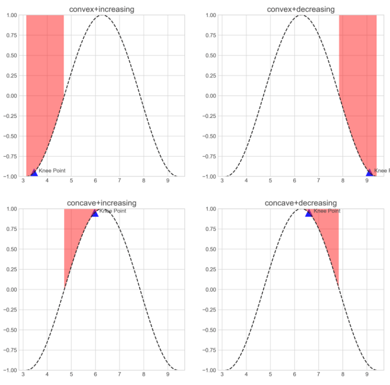
curve:str型,指明曲线之上区域是凸集还是凹集,concave代表凹,convex代表凸
direction:str型,指明曲线初始趋势是增还是减,increasing表示增,decreasing表示减
online:bool型,用于设置在线/离线识别模式,True表示在线,False表示离线;在线模式下会沿着x轴从右向左识别出每一个局部拐点,并在其中选择最优的拐点;离线模式下会返回从右向左检测到的第一个局部拐点
KneeLocator在传入参数实例化完成计算后,可返回的我们主要关注的属性如下:
knee及elbow:返回检测到的最优拐点对应的x
knee_y及elbow_y:返回检测到的最优拐点对应的y
all_elbows及all_knees:返回检测到的所有局部拐点对应的x
all_elbows_y及all_knees_y:返回检测到的所有局部拐点对应的y
import matplotlib.pyplot as pltfrom matplotlib import styleimport numpy as npfrom kneed import KneeLocatorstyle.use('seaborn-whitegrid')x = np.arange(1, 3, 0.01)*np.piy = np.cos(x)# 计算各种参数组合下的拐点kneedle_cov_inc = KneeLocator(x,y,curve='convex',direction='increasing',online=True)kneedle_cov_dec = KneeLocator(x,y,curve='convex',direction='decreasing',online=True)kneedle_con_inc = KneeLocator(x,y,curve='concave',direction='increasing',online=True)kneedle_con_dec = KneeLocator(x,y,curve='concave',direction='decreasing',online=True)fig, axe = plt.subplots(2, 2, figsize=[12, 12])axe[0, 0].plot(x, y, 'k--')axe[0, 0].annotate(s='Knee Point', xy=(kneedle_cov_inc.knee+0.2, kneedle_cov_inc.knee_y), fontsize=10)axe[0, 0].scatter(x=kneedle_cov_inc.knee, y=kneedle_cov_inc.knee_y, c='b', s=200, marker='^', alpha=1)axe[0, 0].set_title('convex+increasing')axe[0, 0].fill_between(np.arange(1, 1.5, 0.01)*np.pi, np.cos(np.arange(1, 1.5, 0.01)*np.pi), 1, alpha=0.5, color='red')axe[0, 0].set_ylim(-1, 1)axe[0, 1].plot(x, y, 'k--')axe[0, 1].annotate(s='Knee Point', xy=(kneedle_cov_dec.knee+0.2, kneedle_cov_dec.knee_y), fontsize=10)axe[0, 1].scatter(x=kneedle_cov_dec.knee, y=kneedle_cov_dec.knee_y, c='b', s=200, marker='^', alpha=1)axe[0, 1].fill_between(np.arange(2.5, 3, 0.01)*np.pi, np.cos(np.arange(2.5, 3, 0.01)*np.pi), 1, alpha=0.5, color='red')axe[0, 1].set_title('convex+decreasing')axe[0, 1].set_ylim(-1, 1)axe[1, 0].plot(x, y, 'k--')axe[1, 0].annotate(s='Knee Point', xy=(kneedle_con_inc.knee+0.2, kneedle_con_inc.knee_y), fontsize=10)axe[1, 0].scatter(x=kneedle_con_inc.knee, y=kneedle_con_inc.knee_y, c='b', s=200, marker='^', alpha=1)axe[1, 0].fill_between(np.arange(1.5, 2, 0.01)*np.pi, np.cos(np.arange(1.5, 2, 0.01)*np.pi), 1, alpha=0.5, color='red')axe[1, 0].set_title('concave+increasing')axe[1, 0].set_ylim(-1, 1)axe[1, 1].plot(x, y, 'k--')axe[1, 1].annotate(s='Knee Point', xy=(kneedle_con_dec.knee+0.2, kneedle_con_dec.knee_y), fontsize=10)axe[1, 1].scatter(x=kneedle_con_dec.knee, y=kneedle_con_dec.knee_y, c='b', s=200, marker='^', alpha=1)axe[1, 1].fill_between(np.arange(2, 2.5, 0.01)*np.pi, np.cos(np.arange(2, 2.5, 0.01)*np.pi), 1, alpha=0.5, color='red')axe[1, 1].set_title('concave+decreasing')axe[1, 1].set_ylim(-1, 1)# 导出图像plt.savefig('图2.png', dpi=300)

若有收获,就点个赞吧
0 人点赞
