网络图绘制

R 可视化 网络图
使用「ggplot2」来构建数据绘制网络图，下面来看具体案例操作

安装并加载R包

package.list=c("tidyverse","magrittr","patchwork")
for (package in package.list) {
  if (!require(package,character.only=T, quietly=T)) {
    install.packages(package)
    library(package, character.only=T)
  }
}

导入数据构建数据集

plot_data <- read_tsv("data.xls") %>% 
  mutate(theta = seq(0,2 * pi, length.out = 100),x = 10 * cos(theta),
         y = 10 * sin(theta),labx = 12 * cos(theta),
         laby = 12 * sin(theta),angle = 360*(theta/(2*pi)))

数据清洗

Creativity <- plot_data %>%
  filter(category == "Creativity") %>%
  select(x, y) %>%
  mutate(id = row_number())
Creativity_edges <- tibble(expand.grid(id1 = Creativity$id, id2 = Creativity$id)) %>%
  inner_join(Creativity, by = c("id1" = "id")) %>%
  inner_join(Creativity, by = c("id2" = "id")) %>%
  select(-c(id1, id2)) %>%
  set_colnames(c("x", "y", "xend", "yend"))
Identity <- plot_data %>%
  filter(category == "Identity") %>%
  select(x, y) %>%
  mutate(id = row_number())
Identity_edges <- tibble(expand.grid(id1 = Identity$id, id2 = Identity$id)) %>%
  inner_join(Identity, by = c("id1" = "id")) %>%
  inner_join(Identity, by = c("id2" = "id")) %>%
  select(-c(id1, id2)) %>%
  set_colnames(c("x", "y", "xend", "yend"))

数据可视化1

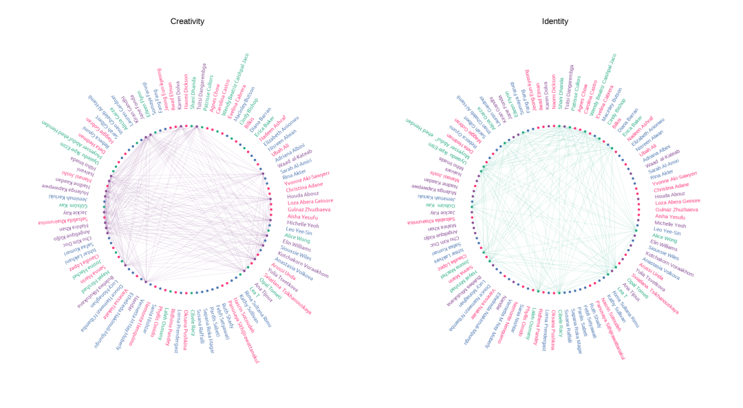
p1 <- ggplot() +
  geom_segment(data = Creativity_edges,mapping = aes(x = x, y = y, xend = xend, yend = yend),
               colour = alpha("#884c94", 0.5), size = 0.05) +
  geom_point(data = plot_data,mapping = aes(x = x, y = y, colour = category),size =1) +
  geom_text(data = plot_data,
            mapping = aes(x = labx, y = laby, label = name, angle = angle, colour = category),
            family = "ubuntu", hjust = 0, size =4) +
  scale_colour_manual("", values = c("white", "#884c94", "#26aa83", "#4a75b0", "#ff3377")) +
  labs(subtitle = "Creativity") +xlim(-20, 20) +
  ylim(-20, 20) +
  coord_fixed() +
  theme_void() +
  theme(legend.position = "none",
        legend.text = element_text(hjust = 0.5, size = 12, color = "white"),
        plot.subtitle = element_text(hjust = 0.5, size = 18, color = "black"),
        plot.background = element_rect(fill = "white", colour="white"),
        panel.background = element_rect(fill = "white", colour="white"),
        plot.margin = unit(c(0,0,0,0), "cm"))

数据可视化2

p2 <- ggplot() +
  geom_segment(data = Identity_edges,mapping = aes(x = x, y = y, xend = xend, yend = yend),
               colour = alpha("#26aa83",0.5), size = 0.05) +
  geom_point(data = plot_data,mapping = aes(x = x, y = y, colour = category),size = 1) +
  geom_text(data = plot_data,
            mapping = aes(x = labx, y = laby, label = name, angle = angle, colour = category),
            hjust = 0,size =4) +
  scale_colour_manual("", values = c("white","#884c94", "#26aa83", "#4a75b0","#ff3377")) +
  labs(subtitle = "Identity") +
  xlim(-20, 20) +
  ylim(-20, 20) +
  coord_fixed() +
  theme_void() +
  theme(legend.position = "none",
        plot.subtitle = element_text(hjust = 0.5, size = 18, color = "black"),
        plot.background = element_rect(fill = "white", colour="white"),
        panel.background = element_rect(fill = "white", colour="white"),
        plot.margin = unit(c(0,0,0,0), "cm"))

拼图

p1 + p2 +
  theme(
        plot.background = element_rect(fill = "white", colour="white"),
        panel.background = element_rect(fill = "white", colour="white"))