未编译的压缩包
randomforest-matlab.zip
这个压缩包中包含:回归和分类两部分的代码,具体的文件如下图1所示
图1. 未编译文件列表
在使用这部分文件的时候,直接运行图中的tutorial_ClassRF.m这个教程文件,但是会出现mex编译文件的错误,这部分目前还没有解决。
解决办法
mex编译文件是c/c++与matlab混编过程中用到的,主要是让matlab能够调用c/c++的文件,加快运行速度
在Microsoft Visual Studio中开发Matlab的mexw文件,生成mexw64或mexw32文件,教程
已编译的压缩包
所以直接使用已经预编译完成的文件夹,Windows-Precompiled-RF_MexStandalone-v0.02-.zip
其中的文件列表如图2所示:
图2. 预编译完成的文件夹
直接进入tutorial_ClassRF.m文件,代码如下
% A simple tutorial file to interface with RF% Options copied from http://cran.r-project.org/web/packages/randomForest/randomForest.pdf%run plethora of testsclcclose all%compile everythingif strcmpi(computer,'PCWIN') |strcmpi(computer,'PCWIN64')compile_windowselsecompile_linuxendtotal_train_time=0;total_test_time=0;%load the twonorm datasetload data/twonorm%modify so that training data is NxD and labels are Nx1, where N=#of%examples, D=# of featuresX = inputs';Y = outputs;[N D] =size(X);%randomly split into 250 examples for training and 50 for testingrandvector = randperm(N);X_trn = X(randvector(1:250),:);Y_trn = Y(randvector(1:250));X_tst = X(randvector(251:end),:);Y_tst = Y(randvector(251:end));% example 1: simply use with the defaultsmodel = classRF_train(X_trn,Y_trn);Y_hat = classRF_predict(X_tst,model);fprintf('\nexample 1: error rate %f\n', length(find(Y_hat~=Y_tst))/length(Y_tst));% example 2: set to 100 treesmodel = classRF_train(X_trn,Y_trn, 100);Y_hat = classRF_predict(X_tst,model);fprintf('\nexample 2: error rate %f\n', length(find(Y_hat~=Y_tst))/length(Y_tst));% example 3: set to 100 trees, mtry = 2model = classRF_train(X_trn,Y_trn, 100,2);Y_hat = classRF_predict(X_tst,model);fprintf('\nexample 3: error rate %f\n', length(find(Y_hat~=Y_tst))/length(Y_tst));% example 4: set to defaults trees and mtry by specifying values as 0model = classRF_train(X_trn,Y_trn, 0, 0);Y_hat = classRF_predict(X_tst,model);fprintf('\nexample 4: error rate %f\n', length(find(Y_hat~=Y_tst))/length(Y_tst));% example 5: set sampling without replacement (default is with replacement)extra_options.replace = 0 ;model = classRF_train(X_trn,Y_trn, 100, 4, extra_options);Y_hat = classRF_predict(X_tst,model);fprintf('\nexample 5: error rate %f\n', length(find(Y_hat~=Y_tst))/length(Y_tst));% example 6: Using classwt (priors of classes)clear extra_options;extra_options.classwt = [1 1]; %for the [-1 +1] classses in twonorm% if you sort the labels in training and arrange in ascending order then% for twonorm you have -1 and +1 classes, with here assigning 1 to% both classes% As you have specified the classwt above, what happens that the priors are considered% also is considered the freq of the labels in the data. If you are% confused look into src/rfutils.cpp in normClassWt() functionmodel = classRF_train(X_trn,Y_trn, 100, 4, extra_options);Y_hat = classRF_predict(X_tst,model);fprintf('\nexample 6: error rate %f\n', length(find(Y_hat~=Y_tst))/length(Y_tst));% example 7: modify to make class(es) more IMPORTANT than the others% extra_options.cutoff (Classification only) = A vector of length equal to% number of classes. The 'winning' class for an observation is the one with the maximum ratio of proportion% of votes to cutoff. Default is 1/k where k is the number of classes (i.e., majority% vote wins). clear extra_options;extra_options.cutoff = [1/4 3/4]; %for the [-1 +1] classses in twonorm% if you sort the labels in training and arrange in ascending order then% for twonorm you have -1 and +1 classes, with here assigning 1/4 and% 3/4 respectively% thus the second class needs a lot less votes to win compared to the first classmodel = classRF_train(X_trn,Y_trn, 100, 4, extra_options);Y_hat = classRF_predict(X_tst,model);fprintf('\nexample 7: error rate %f\n', length(find(Y_hat~=Y_tst))/length(Y_tst));fprintf(' y_trn is almost 50/50 but y_hat now has %f/%f split\n',length(find(Y_hat~=-1))/length(Y_tst),length(find(Y_hat~=1))/length(Y_tst));% extra_options.strata = (not yet stable in code) variable that is used for stratified% sampling. I don't yet know how this works.% example 8: sampsize example% extra_options.sampsize = Size(s) of sample to draw. For classification,% if sampsize is a vector of the length the number of strata, then sampling is stratified by strata,% and the elements of sampsize indicate the numbers to be drawn from the strata.clear extra_optionsextra_options.sampsize = size(X_trn,1)*2/3;model = classRF_train(X_trn,Y_trn, 100, 4, extra_options);Y_hat = classRF_predict(X_tst,model);fprintf('\nexample 8: error rate %f\n', length(find(Y_hat~=Y_tst))/length(Y_tst));% example 9: nodesize% extra_options.nodesize = Minimum size of terminal nodes. Setting this number larger causes smaller trees% to be grown (and thus take less time). Note that the default values are different% for classification (1) and regression (5).clear extra_optionsextra_options.nodesize = 2;model = classRF_train(X_trn,Y_trn, 100, 4, extra_options);Y_hat = classRF_predict(X_tst,model);fprintf('\nexample 9: error rate %f\n', length(find(Y_hat~=Y_tst))/length(Y_tst));% example 10: calculating importanceclear extra_optionsextra_options.importance = 1; %(0 = (Default) Don't, 1=calculate)model = classRF_train(X_trn,Y_trn, 100, 4, extra_options);Y_hat = classRF_predict(X_tst,model);fprintf('\nexample 10: error rate %f\n', length(find(Y_hat~=Y_tst))/length(Y_tst));%model will have 3 variables for importance importanceSD and localImp%importance = a matrix with nclass + 2 (for classification) or two (for regression) columns.% For classification, the first nclass columns are the class-specific measures% computed as mean decrease in accuracy. The nclass + 1st column is the% mean decrease in accuracy over all classes. The last column is the mean decrease% in Gini index. For Regression, the first column is the mean decrease in% accuracy and the second the mean decrease in MSE. If importance=FALSE,% the last measure is still returned as a vector.figure('Name','Importance Plots')subplot(2,1,1);bar(model.importance(:,end-1));xlabel('feature');ylabel('magnitude');title('Mean decrease in Accuracy');subplot(2,1,2);bar(model.importance(:,end));xlabel('feature');ylabel('magnitude');title('Mean decrease in Gini index');%importanceSD = The ?standard errors? of the permutation-based importance measure. For classification,% a D by nclass + 1 matrix corresponding to the first nclass + 1% columns of the importance matrix. For regression, a length p vector.model.importanceSD% example 11: calculating local importance% extra_options.localImp = Should casewise importance measure be computed? (Setting this to TRUE will% override importance.)%localImp = a D by N matrix containing the casewise importance measures, the [i,j] element% of which is the importance of i-th variable on the j-th case. NULL if% localImp=FALSE.clear extra_optionsextra_options.localImp = 1; %(0 = (Default) Don't, 1=calculate)model = classRF_train(X_trn,Y_trn, 100, 4, extra_options);Y_hat = classRF_predict(X_tst,model);fprintf('\nexample 11: error rate %f\n', length(find(Y_hat~=Y_tst))/length(Y_tst));model.localImp% example 12: calculating proximity% extra_options.proximity = Should proximity measure among the rows be calculated?clear extra_optionsextra_options.proximity = 1; %(0 = (Default) Don't, 1=calculate)model = classRF_train(X_trn,Y_trn, 100, 4, extra_options);Y_hat = classRF_predict(X_tst,model);fprintf('\nexample 12: error rate %f\n', length(find(Y_hat~=Y_tst))/length(Y_tst));model.proximity% example 13: use only OOB for proximity% extra_options.oob_prox = Should proximity be calculated only on 'out-of-bag' data?clear extra_optionsextra_options.proximity = 1; %(0 = (Default) Don't, 1=calculate)extra_options.oob_prox = 0; %(Default = 1 if proximity is enabled, Don't 0)model = classRF_train(X_trn,Y_trn, 100, 4, extra_options);Y_hat = classRF_predict(X_tst,model);fprintf('\nexample 13: error rate %f\n', length(find(Y_hat~=Y_tst))/length(Y_tst));% example 14: to see what is going on behind the scenes% extra_options.do_trace = If set to TRUE, give a more verbose output as randomForest is run. If set to% some integer, then running output is printed for every% do_trace trees.clear extra_optionsextra_options.do_trace = 1; %(Default = 0)model = classRF_train(X_trn,Y_trn, 100, 4, extra_options);Y_hat = classRF_predict(X_tst,model);fprintf('\nexample 14: error rate %f\n', length(find(Y_hat~=Y_tst))/length(Y_tst));% example 14: to see what is going on behind the scenes% extra_options.keep_inbag Should an n by ntree matrix be returned that keeps track of which samples are% 'in-bag' in which trees (but not how many times, if sampling with replacement)%clear extra_optionsextra_options.keep_inbag = 1; %(Default = 0)model = classRF_train(X_trn,Y_trn, 100, 4, extra_options);Y_hat = classRF_predict(X_tst,model);fprintf('\nexample 15: error rate %f\n', length(find(Y_hat~=Y_tst))/length(Y_tst));model.inbag% example 16: getting the OOB rate. model will have errtr whose first% column is the OOB rate. and the second column is for the 1-st class and% so onmodel = classRF_train(X_trn,Y_trn);Y_hat = classRF_predict(X_tst,model);fprintf('\nexample 16: error rate %f\n', length(find(Y_hat~=Y_tst))/length(Y_tst));figure('Name','OOB error rate');plot(model.errtr(:,1)); title('OOB error rate'); xlabel('iteration (# trees)'); ylabel('OOB error rate');% example 17: getting prediction per tree, votes etc for test setmodel = classRF_train(X_trn,Y_trn);test_options.predict_all = 1;[Y_hat, votes, prediction_pre_tree] = classRF_predict(X_tst,model,test_options);fprintf('\nexample 17: error rate %f\n', length(find(Y_hat~=Y_tst))/length(Y_tst));
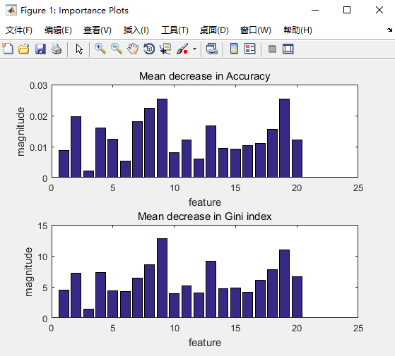
图3. example10结果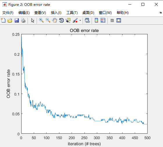
图4. example16结果

若有收获,就点个赞吧
0 人点赞
