项目背景:从链家的网站上,我们获取到一部分房子的交易信息,根据我们感兴趣的因素,进行探索。
数据的探索是随意的。数据清洗考验的是业务理解和细心程度。
处理missing value的时候,一定要小心和严谨,要符合现实生活中的逻辑。
认识数据
加载模块
import numpy as npimport pandas as pdimport seaborn as snsimport matplotlib.pyplot as pltplt.rcParams['font.sans-serif']=['SimHei'] #用来正常显示中文标签plt.rcParams['axes.unicode_minus']=False #用来正常显示负号
原始数据
df = pd.read_excel("bjlianjia.xlsx", 0, header=None)df.head()
| 0 | 1 | 2 | 3 | 4 | 5 | 6 | 7 | 8 | 9 | 10 | 11 | 12 | |
|---|---|---|---|---|---|---|---|---|---|---|---|---|---|
| 0 | 3室1厅1厨1卫 | 2016.08.30 链家成交 | 人定湖北巷 | 750.0 | 东南 北 | 简装 | 1984 | 中楼层 (共6层) | 70年 | 77.5㎡ | 暂无数据 | 无 | 101100406614 |
| 1 | 2室1厅1厨1卫 | 2016.07.31 链家成交 | 刘家窑东里 | 343.0 | 南 西 | 精装 | 1998 | 高楼层 (共18层) | 70年 | 75㎡ | 暂无数据 | 有 | 101091748516 |
| 2 | 3室1厅1厨1卫 | 2017.02.17 链家成交 | 兰园 | 640.0 | 南 北 | 简装 | 1998 | 中楼层 (共6层) | 70年 | 88.1㎡ | 暂无数据 | 无 | 101101151051 |
| 3 | 2室1厅1厨1卫 | 2017.02 其他公司成交 | 科育小区 | NaN | 南 北 | 精装 | 1975 | 顶层 (共4层) | 70年 | 66.69㎡ | 50.03㎡ | 无 | 101100278245 |
| 4 | 3室1厅1厨1卫 | 2016.09.15 链家成交 | 中纺宿舍 | 925.0 | 东南 | 简装 | 未知 | 低楼层 (共18层) | 70年 | 108.86㎡ | 暂无数据 | 有 | 101100449527 |
添加列名
columns = ['房型', '成交时间', '地址', '价格', '朝向', '装修', '建造年代', '楼层', '产权', '面积', '得房面积', '是否有钥匙', '编号']df.columns = columnsdf.head()
| 房型 | 成交时间 | 地址 | 价格 | 朝向 | 装修 | 建造年代 | 楼层 | 产权 | 面积 | 得房面积 | 是否有钥匙 | 编号 | |
|---|---|---|---|---|---|---|---|---|---|---|---|---|---|
| 0 | 3室1厅1厨1卫 | 2016.08.30 链家成交 | 人定湖北巷 | 750.0 | 东南 北 | 简装 | 1984 | 中楼层 (共6层) | 70年 | 77.5㎡ | 暂无数据 | 无 | 101100406614 |
| 1 | 2室1厅1厨1卫 | 2016.07.31 链家成交 | 刘家窑东里 | 343.0 | 南 西 | 精装 | 1998 | 高楼层 (共18层) | 70年 | 75㎡ | 暂无数据 | 有 | 101091748516 |
| 2 | 3室1厅1厨1卫 | 2017.02.17 链家成交 | 兰园 | 640.0 | 南 北 | 简装 | 1998 | 中楼层 (共6层) | 70年 | 88.1㎡ | 暂无数据 | 无 | 101101151051 |
| 3 | 2室1厅1厨1卫 | 2017.02 其他公司成交 | 科育小区 | NaN | 南 北 | 精装 | 1975 | 顶层 (共4层) | 70年 | 66.69㎡ | 50.03㎡ | 无 | 101100278245 |
| 4 | 3室1厅1厨1卫 | 2016.09.15 链家成交 | 中纺宿舍 | 925.0 | 东南 | 简装 | 未知 | 低楼层 (共18层) | 70年 | 108.86㎡ | 暂无数据 | 有 | 101100449527 |
数据清洗
房型数据清洗
df['房型'].value_counts()
2室1厅1厨1卫 498121室1厅1厨1卫 26057- -室- -厅 182163室1厅1厨1卫 130883室2厅1厨2卫 10018...8室4厅1厨4卫 15室2厅2厨1卫 15室4厅1厨2卫 14室1厅1厨0卫 12室2厅1厨4卫 1Name: 房型, Length: 242, dtype: int64
查看房型这一列的数据,是否存在空数据,这很重要(异常处理)
df[df['房型'].isnull()]
| 房型 | 成交时间 | 地址 | 价格 | 朝向 | 装修 | 建造年代 | 楼层 | 产权 | 面积 | 得房面积 | 是否有钥匙 | 编号 | |
|---|---|---|---|---|---|---|---|---|---|---|---|---|---|
| 69 | NaN | NaN | NaN | NaN | NaN | NaN | NaN | NaN | NaN | NaN | NaN | NaN | NaN |
你知道3室1厅1厨1卫 比 1室1厅1厨1卫好,可是怎么才能让计算机也知道呢?
思路一:适当情况下,将字符串转化为数字进行比较
延伸:数值型的数据和非数值型的数据要分开来才好比较
def _parseHouse(s):try:s = s.strip()if (len(s) == 8):return [s[0], s[2], s[4], s[6]]else:return [-1, -1, -1, -1]except:return [-1, -1, -1, -1]room_df = pd.DataFrame(df['房型'].apply(lambda s: _parseHouse(s)).values.tolist(), columns=['室', '厅', '厨', '卫'])# 替换掉无效字符room_df.replace({'-': -1}, inplace=True)room_df.head()
| 室 | 厅 | 厨 | 卫 | |
|---|---|---|---|---|
| 0 | 3 | 1 | 1 | 1 |
| 1 | 2 | 1 | 1 | 1 |
| 2 | 3 | 1 | 1 | 1 |
| 3 | 2 | 1 | 1 | 1 |
| 4 | 3 | 1 | 1 | 1 |
对上面的 tolist 方法作一个简单的解释,请看下面的示例
pd.Series([1, 2, 3, 4]).values # array([1, 2, 3, 4])pd.Series([1, 2, 3, 4]).values.tolist() # [1, 2, 3, 4]
朝向处理
思路二:整合某个数据项的时候,可以对它作拆散处理
接收数据要有异常处理的思维
def _parseCX(s):try:s = s.strip()return s.split(' ')except:return ['unknown']cx_data = df['朝向'].apply(lambda s: _parseCX(s)).values.tolist()cx_data
执行(这里显示的输出结果,由于数据量太大,作了一定的简化处理)
[['东南', '北'],['南', '西'],['南', '北'],['南', '北'],['东南'],['东南', '北'],['南', '北'],['南', '北'],['东', '西'],['东南'],['南'],['南', '北'],...['南', '北'],['南', '西'],['暂无数据'],['南', '北'],...]
成交时间处理
import re# 匹配数字和特殊符号.re.compile("[\d|\.]+").findall(df['成交时间'][0])[0] # '2016.08.30'
思路三:时间年月日通常是入手的一个维度,或时间的差值,小时数
这里我们提取时间,因为针对价格而言,季度之间还是有区别的
import re

def _parseDate(s):
    try:
        p = re.compile("[\d\.]+")
        return p.findall(s)[0]
    except:
        return "-1.-1.-1"

date_df = df['成交时间'].apply(lambda s: _parseDate(s))
date_df = pd.DataFrame(date_df.apply(lambda s: s.split('.')).values.tolist(), columns=['年', '月', '日'])

# 有些数据项只记录了年和月,没有具体日期,所以我们需要处理空值
date_df.fillna(-1, inplace=True)

date_df.head()
| 年 | 月 | 日 | |
|---|---|---|---|
| 0 | 2016 | 08 | 30 |
| 1 | 2016 | 07 | 31 |
| 2 | 2017 | 02 | 17 |
| 3 | 2017 | 02 | -1 |
| 4 | 2016 | 09 | 15 |
产权面积处理
print(re.compile("[\d|\.]+").findall(df['产权'][0])[0])    # 70
print(re.compile("[\d|\.]+").findall(df['面积'][0])[0])    # 77.5
同样是拆分数字和字符串,与上面的思路相同
import re

def _parseArea(s):
    try:
        p = re.compile("[\d]+")
        return p.findall(s)[0]
    except:
        return -1

area_df = df['面积'].apply(lambda s: _parseArea(s))
property_df = df['产权'].apply(lambda s: _parseArea(s))

area_df.value_counts().sort_values(ascending=False)[:10]
查看下交易量前10的房子面积是多少?
57    4431
58    3910
61    3484
60    3289
54    3228
56    3040
59    2868
62    2729
55    2628
63    2548
Name: 面积, dtype: int64
我们可以看到,在当前的数据集内,交易量最大的房型面积为57平米,大多在五十多到六十多平方米。
可视化展示
房型探索
fig, axes = plt.subplots(nrows=2, ncols=2)
ax0, ax1, ax2, ax3 = axes.flatten()

# temp = room_df['室'].value_counts().reset_index()
# sns.barplot(x = 'index', y = '室', data=temp, ax=ax0) # ax指定子图的位置

# temp = room_df['厅'].value_counts().reset_index()
# sns.barplot(x = 'index', y = '厅', data=temp, ax=ax1)

# temp = room_df['厨'].value_counts().reset_index()
# sns.barplot(x = 'index', y = '厨', data=temp, ax=ax2)

# temp = room_df['卫'].value_counts().reset_index()
# sns.barplot(x = 'index', y = '卫', data=temp, ax=ax3)

# print(type(axes.flatten()))     # <class 'numpy.ndarray'>
# print(type(room_df.columns))    # <class 'pandas.core.indexes.base.Index'>

map = {'室': 'room', '厅': 'parlour', '厨': 'kitchen', '卫': 'toilet'}

# 使用循环的方式来画图,是较为明智的做法
for ax, col in zip(axes.flatten(), room_df.columns):     # zip函数绑定到一起
    temp = room_df[col].value_counts().reset_index().rename(columns={'index': map.get(col), col: 'frequency'})
    sns.barplot(x = map.get(col), y = 'frequency', data = temp, ax = ax)    # 注意ax参数的用法
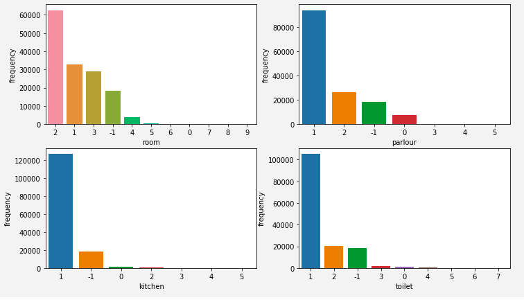
确实是存在9室的房子,可通过 room_df.astype(float64).max() 输出查看。
根据图示我们可以猜测到,2室1厅1厨1卫是最为受欢迎的。但是上面的图示是每个属性独立考虑的,下面我们综合考虑下。
# 过滤掉值为-1的行,为无效数据
temp_room = room_df.replace(-1, np.nan).dropna(how='any')

# 按交易数量排序,取排名前三的
max_room = temp_room.groupby(['室', '厅', '厨', '卫']).size().sort_values(ascending=False)[:3]
max_room = pd.DataFrame(max_room, columns=['frequency'])

# 计算百分比
max_room['percent'] = round(max_room['frequency'] / len(temp_room), 3)
max_room
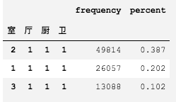
我们可以得出结论:在给定的数据集下,两室一厅一厨一卫的房型卖的最好,占比约为38%。
一室一厅一厨一卫和三室一厅一厨一卫的房型销量分别排名第二第三。
成交价格探索
我们先看下价格这一列数据的分布情况是怎样的
df['价格'].describe()
执行
count    99424.000000
mean       406.940825
std        277.388223
min          0.100000
25%        237.000000
50%        340.000000
75%        498.000000
max      18130.000000
Name: 价格, dtype: float64
中位数为340万,房子都不便宜呀
连续随机变量的分布我们通常通过直方图来查看
# 价格的集中趋势
sns.distplot(df['价格'].fillna(0))
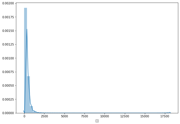
上面这个输出结果实在是差强人意,因为我们对交易价格在2500万以上的房型丝毫不感兴趣,那离我们太遥远了。
思路四:对连续型特征离散化,更直观查看分布
pd.cut(df['价格'].fillna(0), bins=3).reset_index().groupby('价格').size()
价格
(-18.13, 6043.333]       147167
(6043.333, 12086.667]         2
(12086.667, 18130.0]          1
dtype: int64
我们暂时将数据划分成了3个等宽度的区间,可以观察到,有将近15万的房型交易价格在第一个区间内,即在6043万以下。
pd.cut(df['价格'].fillna(0), bins=3).value_counts()
(-18.13, 6043.333]       147167
(6043.333, 12086.667]         2
(12086.667, 18130.0]          1
Name: 价格, dtype: int64
输出结果与上面是等价的,cut方法返回的结果是Series类型。
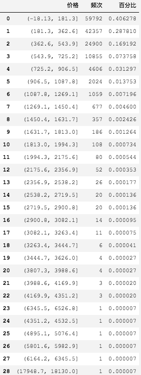
真正的重头戏,有意义的输出来了
cut_price = pd.cut(df['价格'].fillna(0), bins=100).value_counts()

# 因为存在很多价格区间是没有交易数据的,过滤掉
cut_price = pd.DataFrame(cut_price[(cut_price > 0).values.tolist()]).reset_index()

# 使得列名有意义
cut_price.rename(columns={'index': '价格', '价格': '频次'}, inplace=True)

total = sum(cut_price['频次'])
cut_price['百分比'] = cut_price['频次'] / total

cut_price
执行
# 离散型变量,我们作柱状图
cut_price.plot.bar(x='价格', y='频次')

# 注意这个小技巧
# 本来是位置0对应第一个元素,现在变成了x轴上的位置-1对应第一个元素,使倾斜之后的值对应相应的柱子
plt.xticks(range(-1, 28), cut_price['价格'].values, rotation=60)

图中显示的方块是因为没能正确处理中文显示的问题,可暂时性忽略。
我们可以得出结论:在当前的数据集下,有40%的购房者选择了180万以下的房子,有将近30%的购房者,选择了180万到360万之间的房子。
0 - 360万占比将近70%,360万才刚刚是及格线70分呀。
成交时间探索
date_df.groupby(['年', '月']).size().sort_values(ascending=False)
执行
年     月
2016  03    5650
      08    5418
2015  12    4913
2016  09    4691
      01    4488
            ...
2010  07       1
      05       1
      04       1
2007  10       1
2005  06       1
Length: 87, dtype: int64
date_df.groupby(['年']).size().sort_values(ascending=False)
执行
年
2016    43159
2015    40096
2014    19980
2013    19834
2012    12073
2017     9989
2011     2019
2010       10
-1          6
2007        3
2005        1
dtype: int64
date_df.groupby(['年']).size().sort_index().reset_index().plot.bar(x='年', y = 0)
执行
<matplotlib.axes._subplots.AxesSubplot at 0x1a3c893128>
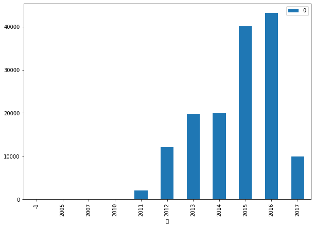
y轴表示交易量,上面代码中之所以选取y=0是因为reset_index之后,column默认从0开始。
从年的角度考虑,我们可以明显看到2015年,2016年,交易量有一个明显的上涨,甚至是翻倍的增长。
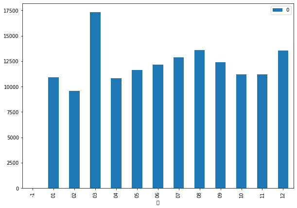
从月的角度考虑,我们可以感觉到,过年后的交易量有一定程度的放大。
date_df.groupby(['月']).size().sort_index().reset_index().plot.bar(x='月', y = 0)
执行
<matplotlib.axes._subplots.AxesSubplot at 0x1a48c10588>
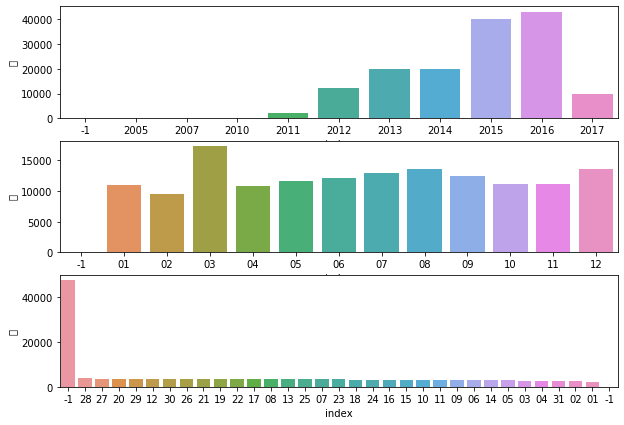
好看漂亮的图来了
fig, axes = plt.subplots(3, 1)

for i, col in enumerate(date_df.columns):
    temp_df = date_df[col].value_counts().reset_index()
    sns.barplot(x="index", y=col, data=temp_df, ax=axes[i])
年销售额
df[['year', 'month']] = date_df[['年', '月']]

data = df.groupby('year').agg({'价格': 'sum'}).reset_index()

sns.barplot(x='year', y='价格', data=data)

data
执行
| year | 价格 | |
|---|---|---|
| 0 | -1 | 0.0 |
| 1 | 2005 | 0.0 |
| 2 | 2007 | 0.0 |
| 3 | 2010 | 663.5 |
| 4 | 2011 | 463515.7 |
| 5 | 2012 | 2984654.2 |
| 6 | 2013 | 4023812.9 |
| 7 | 2014 | 3853053.2 |
| 8 | 2015 | 8969057.4 |
| 9 | 2016 | 14610134.5 |
| 10 | 2017 | 5554793.2 |
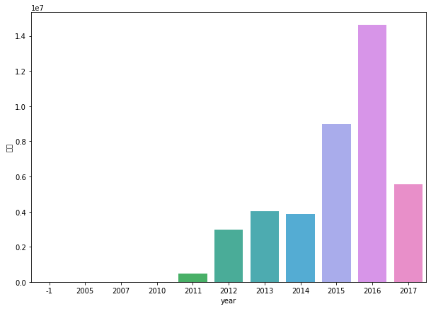
我们可以看到,在2016年销售额达到了一个顶峰,将近快一千五百万了。
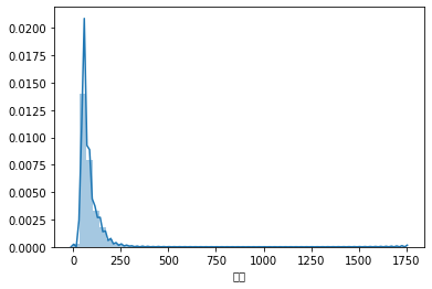
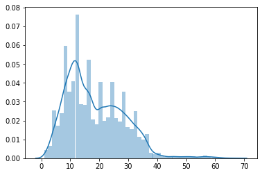
面积探索
# 两行代码同样的效果
# sns.distplot(df['面积'].apply(lambda s: float(_parseArea(s))))

sns.distplot(df['面积'].apply(lambda s: _parseArea(s)).astype('float16'))
执行
<matplotlib.axes._subplots.AxesSubplot at 0x1a21d13ba8>
思路五:截掉尾巴显示
我们可以认为超过200平米的,属于是比较特殊的情况,在可视化时可不显示。
temp_df = df['面积'].apply(lambda s: _parseArea(s)).astype('float')
sns.distplot(temp_df[temp_df <= 200])
执行
<matplotlib.axes._subplots.AxesSubplot at 0x1a2442ad30>
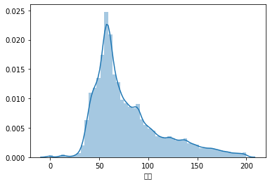
我们可以得出结论:在当前的数据集下,大部分交易房型的面积位于50平方到70平方之间(粗略估计)。
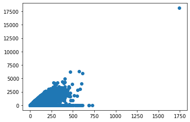
面积与价格的关系
plt.scatter(x=df['面积'].apply(lambda s: _parseArea(s)).astype('float'), y=df['价格'].fillna(0))
执行
<matplotlib.collections.PathCollection at 0x1a239e6668>
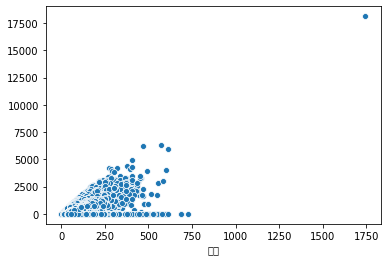
sns.scatterplot(x=df['面积'].apply(lambda s: _parseArea(s)).astype('float'), y=df['价格'].fillna(0))
执行
<matplotlib.axes._subplots.AxesSubplot at 0x1a252009b0>
data = pd.DataFrame(list(zip(df['面积'].apply(lambda s: _parseArea(s)).astype('float'), df['价格'].fillna(0).values)), columns=['area', 'price'])

data.head()
执行
| area | price | |
|---|---|---|
| 0 | 77.0 | 750.0 |
| 1 | 75.0 | 343.0 |
| 2 | 88.0 | 640.0 |
| 3 | 66.0 | 0.0 |
| 4 | 108.0 | 925.0 |
data = data[data['area'] < 200]
sns.jointplot(x='area', y='price', data=data)
执行
<seaborn.axisgrid.JointGrid at 0x1a22c7a860>
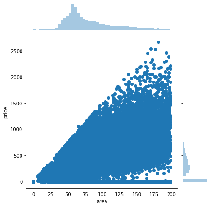
上面我们通过三种不同方式输出的图形都表明,面积与价格没有显著的线性关系。
新旧程度探索
# date_df['年'] - df['建造年代'].apply(lambda s: str(s)).replace({'未知', -1}).astype('int')

init = df['建造年代'].apply(lambda s: str(s).strip()).replace({'未知': -1}).fillna(-1)

diff_df = date_df['年'].astype('float16') - init.astype('float16')

diff_df = diff_df[(diff_df > 0) & (diff_df < 70)]

sns.distplot(diff_df)
执行
<matplotlib.axes._subplots.AxesSubplot at 0x1a2fa2b400>
因为国内大部分房子的产权都是70年,所以我们没必要考虑70年以前建造的房子了。
我们得出结论:在当前的数据集下,大部分的交易房型修建年代在十一或十二年前。

若有收获,就点个赞吧
0 人点赞
