背景简介
摩拜单车自推出以来,深受用户喜爱,在很多城市已经成为除公共交通以外的居民首选的 出行方式,大大减轻了城市路网压力和拥堵情况。随着绿色出行和环保观念的深入人心, 将会有更多的用户选择摩拜单车,进一步实现让自行车回归城市的目标。同时,摩拜致力于应用前沿科技的帮助人们更好地出行,利用机器学习去预测用户的出行目的地便是众多 应用场景中重要的一个。
目前,摩拜单车在北京的单车投放量已经超过40万。用户可以直接在人行道上找到停放的单车,用手机解锁,然后骑到目的地后再把单车停好并锁上。因此,为了更好地调配和管理这40万辆单车,需要准确地预测每个用户的骑行目的地。
任务描述
参赛者需要根据摩拜提供的数据,预测骑行的目的地所在区块。
比赛地训练集取北京某一区域的一段时间内的部分数据,测试集为同一区域未来一段时间的数据。训练集的将划分为public set和private set划分。比赛过程中,选手将只能看到public set的分数,但比赛的最终排名将由private set的分数决定。
标注数据中包含300万条出行记录数据,覆盖超过30万用户和40万摩拜单车。数据包括骑行起始时间和地点、车辆ID、车辆类型和用户ID等信息。参赛选手需要预测骑行目的地的区块位置。
认识数据
加载模块
import pandas as pdimport seaborn as snsimport geohash # 需要将脚本文件geohash.sh置于当前目录下import matplotlib.pyplot as pltfrom math import radians, cos, sin, asin, sqrt
初探数据
# parase_date是有作用的,将字符串类型转换成了Timestamp类型train = pd.read_csv('train.csv', sep=',', parse_dates=['starttime'])test = pd.read_csv('test.csv', sep=',', parse_dates=['starttime'])train.head()
| orderid | userid | bikeid | biketype | starttime | geohashed_start_loc | geohashed_end_loc | |
|---|---|---|---|---|---|---|---|
| 0 | 1893973 | 451147 | 210617 | 2 | 2017-05-14 22:16:50 | wx4snhx | wx4snhj |
| 1 | 4657992 | 1061133 | 465394 | 1 | 2017-05-14 22:16:52 | wx4dr59 | wx4dquz |
| 2 | 2965085 | 549189 | 310572 | 1 | 2017-05-14 22:16:51 | wx4fgur | wx4fu5n |
| 3 | 4548579 | 489720 | 456688 | 1 | 2017-05-14 22:16:51 | wx4d5r5 | wx4d5r4 |
| 4 | 3936364 | 467449 | 403224 | 1 | 2017-05-14 22:16:50 | wx4g27p | wx4g266 |
test.head()
| orderid | userid | bikeid | biketype | starttime | geohashed_start_loc | |
|---|---|---|---|---|---|---|
| 0 | 86458 | 467987 | 13488 | 1 | 2017-05-27 19:19:41 | wx4gfbe |
| 1 | 1473189 | 976462 | 170537 | 2 | 2017-05-31 17:45:38 | wx4eqep |
| 2 | 1441027 | 790813 | 167447 | 2 | 2017-05-26 11:31:48 | wx4e5zr |
| 3 | 4747983 | 744823 | 472963 | 1 | 2017-05-31 18:30:43 | wx4dxz4 |
| 4 | 43984 | 712391 | 7158 | 1 | 2017-05-25 12:46:16 | wx4ewq5 |
print(train.shape) # (3214096, 7)print(test.shape) # (2002996, 6)
因为数据量太大(321万条数据),为了使模型更快的跑出结果,我们可以考虑减少一半的数据量,即进行随机抽样操作。(这个操作可以根据需要做或不做,我自己在实践的时候,取的是全部的数据。)
train = train.sample(frac=0.5) # 随机50%
认识GeoHash
抛出问题
点外卖的时候软件是怎么返回最近的餐馆的?难道是每个餐馆和用户之间计算距离排序吗?(这样的计算量着实太大,毕竟用户太多,餐馆太多)
一个好的解决方案是分区块,想象一个三行三列的表格,只返回周边的8个块和自身的一个块内的餐馆数据。
那只返回一个区块内的餐馆行不行?我们考虑下面这种情况(红点表示用户的位置,黑点表示餐馆的位置),很明显,1,2,4区块内相较于区块5存在距离用户更近的餐馆,我们应该优先返回。

解决方案
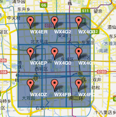
- GeoHash将二维的经纬度转换成字符串,比如下图展示了北京9个区域的GeoHash字符串,分别是WX4ER,WX4G2、WX4G3等等,每一个字符串代表了某一矩形区域。也就是说,这个矩形区域内所有的点(经纬度坐标)都共享相同的GeoHash字符串,这样既可以保护隐私(只表示大概区域位置而不是具体的点),又比较容易做缓存,比如左上角这个区域内的用户不断发送位置信息请求餐馆数据,由于这些用户的GeoHash字符串都是WX4ER,所以可以把WX4ER当作key,把该区域的餐馆信息当作value来进行缓存,而如果不使用GeoHash的话,由于区域内的用户传来的经纬度是各不相同的,很难做缓存。
- 字符串越长,表示的范围越精确。如图所示,5位的编码能表示10平方千米范围的矩形区域,而6位编码能表示更精细的区域(约0.34平方千米)
字符串相似的表示距离相近,这样可以利用字符串的前缀匹配来查询附近的POI信息
数据清洗
时间处理
我们想,根据正常的逻辑,用户出行肯定存在早晚高峰,工作日与非工作日的出行规律肯定也不一样。
# 0 Monday 6 Sundaytrain['weekday'] = train['starttime'].apply(lambda t: t.weekday())train['hour'] = train['starttime'].apply(lambda t: t.hour)train['day'] = train['starttime'].apply(lambda t: str(t)[:10])train.head()
| orderid | userid | bikeid | biketype | starttime | geohashed_start_loc | geohashed_end_loc | weekday | hour | day | |
|---|---|---|---|---|---|---|---|---|---|---|
| 0 | 1893973 | 451147 | 210617 | 2 | 2017-05-14 22:16:50 | wx4snhx | wx4snhj | 6 | 22 | 2017-05-14 |
| 1 | 4657992 | 1061133 | 465394 | 1 | 2017-05-14 22:16:52 | wx4dr59 | wx4dquz | 6 | 22 | 2017-05-14 |
| 2 | 2965085 | 549189 | 310572 | 1 | 2017-05-14 22:16:51 | wx4fgur | wx4fu5n | 6 | 22 | 2017-05-14 |
| 3 | 4548579 | 489720 | 456688 | 1 | 2017-05-14 22:16:51 | wx4d5r5 | wx4d5r4 | 6 | 22 | 2017-05-14 |
| 4 | 3936364 | 467449 | 403224 | 1 | 2017-05-14 22:16:50 | wx4g27p | wx4g266 | 6 | 22 | 2017-05-14 |
通常情况下,我们并不直接修改原始数据,我们把数据copy给另一个变量。
kv = dict()for a, b in zip(list(range(7)), ['周一','周二','周三','周四','周五','周六','周日']):kv[a] = bdf = train.loc[:,:'geohashed_end_loc']df['date'] = train['day']df['weekday'] = train['weekday'].apply(lambda d: kv.get(d))df['hour'] = train['hour'].apply(lambda h: str(h) + '时')df.head()
| orderid | userid | bikeid | biketype | starttime | geohashed_start_loc | geohashed_end_loc | date | weekday | hour | |
|---|---|---|---|---|---|---|---|---|---|---|
| 0 | 1893973 | 451147 | 210617 | 2 | 2017-05-14 22:16:50 | wx4snhx | wx4snhj | 2017-05-14 | 周日 | 22时 |
| 1 | 4657992 | 1061133 | 465394 | 1 | 2017-05-14 22:16:52 | wx4dr59 | wx4dquz | 2017-05-14 | 周日 | 22时 |
| 2 | 2965085 | 549189 | 310572 | 1 | 2017-05-14 22:16:51 | wx4fgur | wx4fu5n | 2017-05-14 | 周日 | 22时 |
| 3 | 4548579 | 489720 | 456688 | 1 | 2017-05-14 22:16:51 | wx4d5r5 | wx4d5r4 | 2017-05-14 | 周日 | 22时 |
| 4 | 3936364 | 467449 | 403224 | 1 | 2017-05-14 22:16:50 | wx4g27p | wx4g266 | 2017-05-14 | 周日 | 22时 |
区块decode
数据集中只记录了用户起始和终止的区块位置信息,这样子我们是没有办法计算用户的出行距离的。要想计算出行距离,就得将区块转换成经纬度,这样子才好计算距离。
我们之前导入的脚本geohash.sh就是用来干这个事情的。
df['start_lat_lng'] = df['geohashed_start_loc'].apply(lambda s: geohash.decode(s))df.head()
| orderid | userid | bikeid | biketype | starttime | geohashed_start_loc | geohashed_end_loc | date | weekday | hour | start_lat_lng | |
|---|---|---|---|---|---|---|---|---|---|---|---|
| 0 | 1893973 | 451147 | 210617 | 2 | 2017-05-14 22:16:50 | wx4snhx | wx4snhj | 2017-05-14 | 周日 | 22时 | (40.10353088378906, 116.28959655761719) |
| 1 | 4657992 | 1061133 | 465394 | 1 | 2017-05-14 22:16:52 | wx4dr59 | wx4dquz | 2017-05-14 | 周日 | 22时 | (39.79042053222656, 116.32530212402344) |
| 2 | 2965085 | 549189 | 310572 | 1 | 2017-05-14 22:16:51 | wx4fgur | wx4fu5n | 2017-05-14 | 周日 | 22时 | (39.88243103027344, 116.54228210449219) |
| 3 | 4548579 | 489720 | 456688 | 1 | 2017-05-14 22:16:51 | wx4d5r5 | wx4d5r4 | 2017-05-14 | 周日 | 22时 | (39.76570129394531, 116.16325378417969) |
| 4 | 3936364 | 467449 | 403224 | 1 | 2017-05-14 22:16:50 | wx4g27p | wx4g266 | 2017-05-14 | 周日 | 22时 | (39.96345520019531, 116.38847351074219) |
df['end_lat_lng'] = df['geohashed_end_loc'].apply(lambda s: geohash.decode(s))
对终点也作一个区块字符串的decode操作。
区块邻居
摩拜单车的定位是短途出行,用户有没有可能只是骑到了邻边的区块呢?(这一点不容易想到,可能需要一定的经验)
df['start_neighbors'] = df['geohashed_start_loc'].apply(lambda n: geohash.neighbors(n))
区块扩大(6)
上面我们已经知道,6位编码的区块距离大约在0.34平方千米,数据集中的区块编码是7位,如果用户骑车超过了7位编码的邻边区块,那有没有超过6位编码的邻边区块呢?(区块的范围更大了,编码越少范围越大)
df['geohashed_start_loc_6'] = df['geohashed_start_loc'].apply(lambda s: s[:6])df['geohashed_end_loc_6'] = df['geohashed_end_loc'].apply(lambda s: s[:6])df['start_neighbors_6'] = df['geohashed_start_loc_6'].apply(lambda s: geohash.neighbors(s))df.head()
| orderid | userid | bikeid | biketype | starttime | geohashed_start_loc | geohashed_end_loc | date | weekday | hour | start_lat_lng | end_lat_lng | start_neighbors | geohashed_start_loc_6 | geohashed_end_loc_6 | start_neighbors_6 | |
|---|---|---|---|---|---|---|---|---|---|---|---|---|---|---|---|---|
| 0 | 1893973 | 451147 | 210617 | 2 | 2017-05-14 22:16:50 | wx4snhx | wx4snhj | 2017-05-14 | 周日 | 22时 | (40.10353088378906, 116.28959655761719) | (40.10078430175781, 116.28684997558594) | [wx4snhw, wx4snk8, wx4snhy, wx4snhz, wx4snkb, … | wx4snh | wx4snh | [wx4sju, wx4snk, wx4sjv, wx4snj, wx4snm, wx4sj… |
| 1 | 4657992 | 1061133 | 465394 | 1 | 2017-05-14 22:16:52 | wx4dr59 | wx4dquz | 2017-05-14 | 周日 | 22时 | (39.79042053222656, 116.32530212402344) | (39.79728698730469, 116.32255554199219) | [wx4dr58, wx4dr5d, wx4dr5b, wx4dr5c, wx4dr5f, … | wx4dr5 | wx4dqu | [wx4dqg, wx4dr7, wx4dqu, wx4drh, wx4drk, wx4dq… |
| 2 | 2965085 | 549189 | 310572 | 1 | 2017-05-14 22:16:51 | wx4fgur | wx4fu5n | 2017-05-14 | 周日 | 22时 | (39.88243103027344, 116.54228210449219) | (39.87556457519531, 116.55189514160156) | [wx4fguq, wx4fuh2, wx4fguw, wx4fgux, wx4fuh8, … | wx4fgu | wx4fu5 | [wx4fgs, wx4fuh, wx4fgt, wx4fgv, wx4fuj, wx4fg… |
| 3 | 4548579 | 489720 | 456688 | 1 | 2017-05-14 22:16:51 | wx4d5r5 | wx4d5r4 | 2017-05-14 | 周日 | 22时 | (39.76570129394531, 116.16325378417969) | (39.76570129394531, 116.16188049316406) | [wx4d5r4, wx4d5rh, wx4d5r6, wx4d5r7, wx4d5rk, … | wx4d5r | wx4d5r | [wx4d5p, wx4d5x, wx4d70, wx4d72, wx4d78, wx4d5… |
| 4 | 3936364 | 467449 | 403224 | 1 | 2017-05-14 22:16:50 | wx4g27p | wx4g266 | 2017-05-14 | 周日 | 22时 | (39.96345520019531, 116.38847351074219) | (39.95933532714844, 116.38160705566406) | [wx4g27n, wx4g2e0, wx4g27q, wx4g27r, wx4g2e2, … | wx4g27 | wx4g26 | [wx4g25, wx4g2e, wx4g2h, wx4g2k, wx4g2s, wx4g2… |
定义一个方法,判断是否在邻居区块(包括中心区块),append方法就是把中心区块添加进来。
def inGeohash(start_geohash, end_geohash, names):names.append(start_geohash)if end_geohash in names:return 1else:return 0# 判断出行目的地是否在7位编码的周边区块(包括自身)df['inside'] = df.apply(lambda s: inGeohash(s['geohashed_start_loc'], s['geohashed_end_loc'], s['start_neighbors']), axis=1)# 判断出行目的地是否在6位编码的周边区块(包括自身)df['inside_6'] = df.apply(lambda s: inGeohash(s['geohashed_start_loc_6'], s['geohashed_end_loc_6'], s['start_neighbors_6']), axis=1)
我们来看一下用户出行目的地在邻居区块的占比为多少?
# 7位编码print(df[df['inside'] != 0].shape[0] / df.shape[0]) # 0.06702942289216003# 6位编码print(df[df['inside_6'] != 0].shape[0] / df.shape[0]) # 0.8145291864337593
打印输出,我们可以看到,目的地在7位编码邻居区块的占比约为6.8%,在6位编码邻居区块的占比约为81.5%。
计算距离
def distance(lon1, lat1, lon2, lat2):# lon1, lat1, lon2, lat2 = [radians(i) for i in [lon1, lat1, lon2, lat2]]lon1, lat1, lon2, lat2 = map(radians, [lon1, lat1, lon2, lat2])dlon = lon2 - lon1dlat = lat2 - lat1a = sin(dlat/2)**2 + cos(lat1) * cos(lat2) * sin(dlon/2)**2c = 2 * asin(sqrt(a))r = 6371return c * r * 1000df['start_end_distance'] = df.apply(lambda s: distance(s['start_lat_lng'][1], s['start_lat_lng'][0], s['end_lat_lng'][1], s['end_lat_lng'][0]), axis = 1)df.head()
| orderid | userid | bikeid | biketype | starttime | geohashed_start_loc | geohashed_end_loc | date | weekday | hour | start_lat_lng | end_lat_lng | start_neighbors | geohashed_start_loc_6 | geohashed_end_loc_6 | start_neighbors_6 | inside | inside_6 | start_end_distance | |
|---|---|---|---|---|---|---|---|---|---|---|---|---|---|---|---|---|---|---|---|
| 0 | 1893973 | 451147 | 210617 | 2 | 2017-05-14 22:16:50 | wx4snhx | wx4snhj | 2017-05-14 | 周日 | 22时 | (40.10353088378906, 116.28959655761719) | (40.10078430175781, 116.28684997558594) | [wx4snhw, wx4snk8, wx4snhy, wx4snhz, wx4snkb, … | wx4snh | wx4snh | [wx4sju, wx4snk, wx4sjv, wx4snj, wx4snm, wx4sj… | 0 | 1 | 384.504518 |
| 1 | 4657992 | 1061133 | 465394 | 1 | 2017-05-14 22:16:52 | wx4dr59 | wx4dquz | 2017-05-14 | 周日 | 22时 | (39.79042053222656, 116.32530212402344) | (39.79728698730469, 116.32255554199219) | [wx4dr58, wx4dr5d, wx4dr5b, wx4dr5c, wx4dr5f, … | wx4dr5 | wx4dqu | [wx4dqg, wx4dr7, wx4dqu, wx4drh, wx4drk, wx4dq… | 0 | 1 | 798.761617 |
| 2 | 2965085 | 549189 | 310572 | 1 | 2017-05-14 22:16:51 | wx4fgur | wx4fu5n | 2017-05-14 | 周日 | 22时 | (39.88243103027344, 116.54228210449219) | (39.87556457519531, 116.55189514160156) | [wx4fguq, wx4fuh2, wx4fguw, wx4fgux, wx4fuh8, … | wx4fgu | wx4fu5 | [wx4fgs, wx4fuh, wx4fgt, wx4fgv, wx4fuj, wx4fg… | 0 | 1 | 1120.638699 |
| 3 | 4548579 | 489720 | 456688 | 1 | 2017-05-14 22:16:51 | wx4d5r5 | wx4d5r4 | 2017-05-14 | 周日 | 22时 | (39.76570129394531, 116.16325378417969) | (39.76570129394531, 116.16188049316406) | [wx4d5r4, wx4d5rh, wx4d5r6, wx4d5r7, wx4d5rk, … | wx4d5r | wx4d5r | [wx4d5p, wx4d5x, wx4d70, wx4d72, wx4d78, wx4d5… | 1 | 1 | 117.377687 |
| 4 | 3936364 | 467449 | 403224 | 1 | 2017-05-14 22:16:50 | wx4g27p | wx4g266 | 2017-05-14 | 周日 | 22时 | (39.96345520019531, 116.38847351074219) | (39.95933532714844, 116.38160705566406) | [wx4g27n, wx4g2e0, wx4g27q, wx4g27r, wx4g2e2, … | wx4g27 | wx4g26 | [wx4g25, wx4g2e, wx4g2h, wx4g2k, wx4g2s, wx4g2… | 0 | 1 | 743.197624 |
区块扩大(5)
df['geohashed_start_loc_5'] = df['geohashed_start_loc'].apply(lambda s: s[:5])df['geohashed_end_loc_5'] = df['geohashed_end_loc'].apply(lambda s: s[:5])df['start_neighbors_5'] = df['geohashed_start_loc_5'].apply(lambda s: geohash.neighbors(s))df['inside_5'] = df.apply(lambda s: inGeohash(s['geohashed_start_loc_5'], s['geohashed_end_loc_5'], s['start_neighbors_5']), axis=1)df.head()
| orderid | userid | bikeid | biketype | starttime | geohashed_start_loc | geohashed_end_loc | date | weekday | hour | … | geohashed_start_loc_6 | geohashed_end_loc_6 | start_neighbors_6 | inside | inside_6 | start_end_distance | geohashed_start_loc_5 | geohashed_end_loc_5 | start_neighbors_5 | inside_5 | |
|---|---|---|---|---|---|---|---|---|---|---|---|---|---|---|---|---|---|---|---|---|---|
| 0 | 1893973 | 451147 | 210617 | 2 | 2017-05-14 22:16:50 | wx4snhx | wx4snhj | 2017-05-14 | 周日 | 22时 | … | wx4snh | wx4snh | [wx4sju, wx4snk, wx4sjv, wx4snj, wx4snm, wx4sj… | 0 | 1 | 384.504518 | wx4sn | wx4sn | [wx4sj, wx4sp, wx4sm, wx4sq, wx4sr, wx4ev, wx4… | 1 |
| 1 | 4657992 | 1061133 | 465394 | 1 | 2017-05-14 22:16:52 | wx4dr59 | wx4dquz | 2017-05-14 | 周日 | 22时 | … | wx4dr5 | wx4dqu | [wx4dqg, wx4dr7, wx4dqu, wx4drh, wx4drk, wx4dq… | 0 | 1 | 798.761617 | wx4dr | wx4dq | [wx4dq, wx4f2, wx4dw, wx4dx, wx4f8, wx4dn, wx4… | 1 |
| 2 | 2965085 | 549189 | 310572 | 1 | 2017-05-14 22:16:51 | wx4fgur | wx4fu5n | 2017-05-14 | 周日 | 22时 | … | wx4fgu | wx4fu5 | [wx4fgs, wx4fuh, wx4fgt, wx4fgv, wx4fuj, wx4fg… | 0 | 1 | 1120.638699 | wx4fg | wx4fu | [wx4ff, wx4fu, wx4g4, wx4g5, wx4gh, wx4fd, wx4… | 1 |
| 3 | 4548579 | 489720 | 456688 | 1 | 2017-05-14 22:16:51 | wx4d5r5 | wx4d5r4 | 2017-05-14 | 周日 | 22时 | … | wx4d5r | wx4d5r | [wx4d5p, wx4d5x, wx4d70, wx4d72, wx4d78, wx4d5… | 1 | 1 | 117.377687 | wx4d5 | wx4d5 | [wx4d4, wx4dh, wx4d6, wx4d7, wx4dk, wx49f, wx4… | 1 |
| 4 | 3936364 | 467449 | 403224 | 1 | 2017-05-14 22:16:50 | wx4g27p | wx4g266 | 2017-05-14 | 周日 | 22时 | … | wx4g27 | wx4g26 | [wx4g25, wx4g2e, wx4g2h, wx4g2k, wx4g2s, wx4g2… | 0 | 1 | 743.197624 | wx4g2 | wx4g2 | [wx4er, wx4g3, wx4ex, wx4g8, wx4g9, wx4ep, wx4… | 1 |
5 rows × 23 columns
df[df['inside_5'] == 1].shape[0] / df.shape[0] # 0.9976478611715394
将近是百分之百了,因为5位编码的区块范围已经是非常大了,大部分用户不会骑行那么远。
至此,我们的数据清洗步骤算是告一段落了
数据清洗是脏活累活,就看谁更加细心,能发掘到更多的信息。
数据分析
时间层面分析
问题一:一天之中不同小时内出发的订单数量有规律吗?
猜想:应该存在早高峰和晚高峰
g1 = df.groupby('hour')# print(g1['orderid'].count().sort_values(ascending=False))# 这两行代码的输出是等价的g1.size().sort_values(ascending=False)
执行
hour7时 31614218时 2902948时 28507817时 27324019时 20919412时 19983116时 17927211时 17236513时 16376815时 15501120时 1517489时 14804714时 13638021时 12722110时 1267966时 12171122时 699055时 2908223时 284890时 133061时 62164时 43972时 37143时 2889dtype: int64
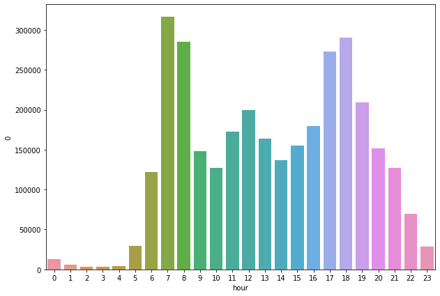
我们可以清楚的观察到:早上七八点和晚上五六点,用户出行达到了一个顶峰。
下面通过图形化的方式来展现一下。
hour_group = df.groupby(['hour'])hour_group = hour_group.size()# 去掉汉字“时”hour_group.index = hour_group.index.str[:-1]hour_group = hour_group.reset_index()# 转为int类型hour_group['hour'] = hour_group['hour'].apply(lambda s: int(s))hour_group = hour_group.sort_values(by = ['hour'], ascending=True)sns.barplot(x='hour', y=0, data=hour_group)
执行
<matplotlib.axes._subplots.AxesSubplot at 0x1be7cbb208>
问题二:工作日与非工作日,用户出行的时间规律相同吗?
猜想:不同,工作日存在早晚高峰,非工作日可能就不存在了。
df['date'].unique()
执行
array(['2017-05-14', '2017-05-15', '2017-05-16', '2017-05-12',
       '2017-05-13', '2017-05-10', '2017-05-11', '2017-05-18',
       '2017-05-19', '2017-05-23', '2017-05-24', '2017-05-20',
       '2017-05-22', '2017-05-21'], dtype=object)
这里需要注意一点:数据集中工作日和非工作日的天数是不同的,我们不能简单的通过类似分析小时出行规律的思路来进行分析(也就是说不能简单的进行求和操作)。
Step 1: 添加一个字段,标志该天是否是周末
# 如果是周末,
df.loc[(df['weekday'] == '周六') | (df['weekday'] == '周日'), 'isWeekend'] = 1
df.loc[~((df['weekday'] == '周六') | (df['weekday'] == '周日')), 'isWeekend'] = 0

g1 = df.groupby(['isWeekend', 'hour'])

# g1['orderid'].count()
# 这两行代码输出的结果是等价的
g1.size()
执行
isWeekend  hour
0.0        0时        8512
           10时      69111
           11时     119007
           12时     148773
           13时     116841
           14时      90993
           15时     103856
           16时     126100
           17时     220159
           18时     230770
           19时     163303
           1时        3865
           20时     116924
           21时      91756
           22时      50128
           23时      20623
           2时        2420
           3时        1915
           4时        3089
           5时       21895
           6时      101157
           7时      273009
           8时      226845
           9时       97571
1.0        0时        4794
           10时      57685
           11时      53358
           12时      51058
           13时      46927
           14时      45387
           15时      51155
           16时      53172
           17时      53081
           18时      59524
           19时      45891
           1时        2351
           20时      34824
           21时      35465
           22时      19777
           23时       7866
           2时        1294
           3时         974
           4时        1308
           5时        7187
           6时       20554
           7时       43133
           8时       58233
           9时       50476
dtype: int64
这样的输出参考意义并不大,因为还是上面我们提到的一点,本身数据集中工作日与非工作日的天数就不同,这样简单的累加是非常不公平的,或许我们可以通过计算平均数来进行分析
Step 2: 计算数据集中工作日与非工作日的天数
g2 = df.groupby(['date', 'weekday'])

w = 0 # 周末天数
c = 0 # 工作日天数

for i, j in list(g2.groups.keys()):
    if j in ['周一','周二','周三','周四','周五']:
        c += 1
    else:
        w += 1
计算结果为工作日c为10天,非工作日w为4天。
Step 3: 计算平均值(给予相同的权重)
temp_df = pd.DataFrame(g1.size()).reset_index()

temp_df.head()
执行
| isWeekend | hour | 0 | |
|---|---|---|---|
| 0 | 0.0 | 0时 | 8512 |
| 1 | 0.0 | 10时 | 69111 |
| 2 | 0.0 | 11时 | 119007 |
| 3 | 0.0 | 12时 | 148773 |
| 4 | 0.0 | 13时 | 116841 |
# 举例,因为统计的是每个工作日0点的订单数,所以除以工作日的天数,就是平均每个工作日0点的订单数
temp_df.loc[temp_df['isWeekend'] == 0.0, 'orderid'] = temp_df[0] / c

temp_df.loc[temp_df['isWeekend'] == 1.0, 'orderid'] = temp_df[0] / w

temp_df.sort_values(['isWeekend', 'orderid'], ascending=False)
执行
| isWeekend | hour | 0 | orderid | |
|---|---|---|---|---|
| 33 | 1.0 | 18时 | 59524 | 14881.00 |
| 46 | 1.0 | 8时 | 58233 | 14558.25 |
| 25 | 1.0 | 10时 | 57685 | 14421.25 |
| 26 | 1.0 | 11时 | 53358 | 13339.50 |
| 31 | 1.0 | 16时 | 53172 | 13293.00 |
| 32 | 1.0 | 17时 | 53081 | 13270.25 |
| 30 | 1.0 | 15时 | 51155 | 12788.75 |
| 27 | 1.0 | 12时 | 51058 | 12764.50 |
| 47 | 1.0 | 9时 | 50476 | 12619.00 |
| 28 | 1.0 | 13时 | 46927 | 11731.75 |
| 34 | 1.0 | 19时 | 45891 | 11472.75 |
| 29 | 1.0 | 14时 | 45387 | 11346.75 |
| 45 | 1.0 | 7时 | 43133 | 10783.25 |
| 37 | 1.0 | 21时 | 35465 | 8866.25 |
| 36 | 1.0 | 20时 | 34824 | 8706.00 |
| 44 | 1.0 | 6时 | 20554 | 5138.50 |
| 38 | 1.0 | 22时 | 19777 | 4944.25 |
| 39 | 1.0 | 23时 | 7866 | 1966.50 |
| 43 | 1.0 | 5时 | 7187 | 1796.75 |
| 24 | 1.0 | 0时 | 4794 | 1198.50 |
| 35 | 1.0 | 1时 | 2351 | 587.75 |
| 42 | 1.0 | 4时 | 1308 | 327.00 |
| 40 | 1.0 | 2时 | 1294 | 323.50 |
| 41 | 1.0 | 3时 | 974 | 243.50 |
| 21 | 0.0 | 7时 | 273009 | 27300.90 |
| 9 | 0.0 | 18时 | 230770 | 23077.00 |
| 22 | 0.0 | 8时 | 226845 | 22684.50 |
| 8 | 0.0 | 17时 | 220159 | 22015.90 |
| 10 | 0.0 | 19时 | 163303 | 16330.30 |
| 3 | 0.0 | 12时 | 148773 | 14877.30 |
| 7 | 0.0 | 16时 | 126100 | 12610.00 |
| 2 | 0.0 | 11时 | 119007 | 11900.70 |
| 12 | 0.0 | 20时 | 116924 | 11692.40 |
| 4 | 0.0 | 13时 | 116841 | 11684.10 |
| 6 | 0.0 | 15时 | 103856 | 10385.60 |
| 20 | 0.0 | 6时 | 101157 | 10115.70 |
| 23 | 0.0 | 9时 | 97571 | 9757.10 |
| 13 | 0.0 | 21时 | 91756 | 9175.60 |
| 5 | 0.0 | 14时 | 90993 | 9099.30 |
| 1 | 0.0 | 10时 | 69111 | 6911.10 |
| 14 | 0.0 | 22时 | 50128 | 5012.80 |
| 19 | 0.0 | 5时 | 21895 | 2189.50 |
| 15 | 0.0 | 23时 | 20623 | 2062.30 |
| 0 | 0.0 | 0时 | 8512 | 851.20 |
| 11 | 0.0 | 1时 | 3865 | 386.50 |
| 18 | 0.0 | 4时 | 3089 | 308.90 |
| 16 | 0.0 | 2时 | 2420 | 242.00 |
| 17 | 0.0 | 3时 | 1915 | 191.50 |
单纯看这个输出的表格,我们可能一时看不出明显的规律,这个时候,就需要我们的可视化工具了。
pylab.rcParams['figure.figsize'] = (10, 7) # 两个参数对应行,列

temp_df['hour'] = temp_df['hour'].str[:-1]

temp_df['hour'] = temp_df['hour'].apply(lambda s: int(s))

temp_df = temp_df.sort_values(['isWeekend', 'hour'], ascending=True)

sns.barplot(x = 'hour', y = 'orderid', hue='isWeekend', data=temp_df)
执行
<matplotlib.axes._subplots.AxesSubplot at 0x1be76e5f28>
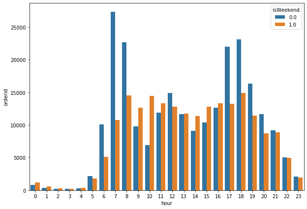
从这个图中我们可以明显看到,周末的出行规律基本上是持平的,不存在什么早晚高峰。只有工作日才存在早晚高峰。
我们得出结论:出行时间和是否是工作日这两个特征,对用户的出行有着重要影响。
距离自身分析
结合项目的目标:预测出行的目的地,那与目的地相关的特征有哪些呢?很重要的一个特征就是:距离
df['distance'] = df['start_end_distance'].apply(lambda s: int(s))
df.head()
执行
| orderid | userid | bikeid | biketype | starttime | geohashed_start_loc | geohashed_end_loc | date | weekday | hour | … | start_neighbors_6 | inside | inside_6 | start_end_distance | geohashed_start_loc_5 | geohashed_end_loc_5 | start_neighbors_5 | inside_5 | isWeekend | distance | |
|---|---|---|---|---|---|---|---|---|---|---|---|---|---|---|---|---|---|---|---|---|---|
| 0 | 1893973 | 451147 | 210617 | 2 | 2017-05-14 22:16:50 | wx4snhx | wx4snhj | 2017-05-14 | 周日 | 22时 | … | [wx4sju, wx4snk, wx4sjv, wx4snj, wx4snm, wx4sj… | 0 | 1 | 384.504518 | wx4sn | wx4sn | [wx4sj, wx4sp, wx4sm, wx4sq, wx4sr, wx4ev, wx4… | 1 | 1.0 | 384 |
| 1 | 4657992 | 1061133 | 465394 | 1 | 2017-05-14 22:16:52 | wx4dr59 | wx4dquz | 2017-05-14 | 周日 | 22时 | … | [wx4dqg, wx4dr7, wx4dqu, wx4drh, wx4drk, wx4dq… | 0 | 1 | 798.761617 | wx4dr | wx4dq | [wx4dq, wx4f2, wx4dw, wx4dx, wx4f8, wx4dn, wx4… | 1 | 1.0 | 798 |
| 2 | 2965085 | 549189 | 310572 | 1 | 2017-05-14 22:16:51 | wx4fgur | wx4fu5n | 2017-05-14 | 周日 | 22时 | … | [wx4fgs, wx4fuh, wx4fgt, wx4fgv, wx4fuj, wx4fg… | 0 | 1 | 1120.638699 | wx4fg | wx4fu | [wx4ff, wx4fu, wx4g4, wx4g5, wx4gh, wx4fd, wx4… | 1 | 1.0 | 1120 |
| 3 | 4548579 | 489720 | 456688 | 1 | 2017-05-14 22:16:51 | wx4d5r5 | wx4d5r4 | 2017-05-14 | 周日 | 22时 | … | [wx4d5p, wx4d5x, wx4d70, wx4d72, wx4d78, wx4d5… | 1 | 1 | 117.377687 | wx4d5 | wx4d5 | [wx4d4, wx4dh, wx4d6, wx4d7, wx4dk, wx49f, wx4… | 1 | 1.0 | 117 |
| 4 | 3936364 | 467449 | 403224 | 1 | 2017-05-14 22:16:50 | wx4g27p | wx4g266 | 2017-05-14 | 周日 | 22时 | … | [wx4g25, wx4g2e, wx4g2h, wx4g2k, wx4g2s, wx4g2… | 0 | 1 | 743.197624 | wx4g2 | wx4g2 | [wx4er, wx4g3, wx4ex, wx4g8, wx4g9, wx4ep, wx4… | 1 | 1.0 | 743 |
5 rows × 25 columns
我们查看一个距离这个特征的描述,比如大部分数据都在什么范围内,有没有很明显的异常值呀
即调用一下describe方法
df['distance'].describe()
执行
count    3.214096e+06
mean     8.142738e+02
std      6.864847e+02
min      1.160000e+02
25%      4.650000e+02
50%      6.600000e+02
75%      9.490000e+02
max      4.490000e+04
Name: distance, dtype: float64
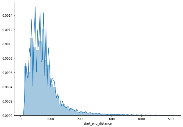
我们可以看到,在当前的数据集下,有75%的用户出行距离在950米以内,平均的出行距离在814米。
sns.distplot(df['start_end_distance'])
执行
<matplotlib.axes._subplots.AxesSubplot at 0x1be7e00550>
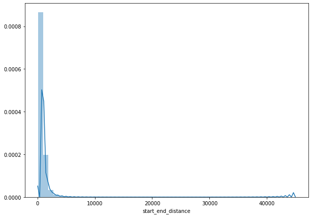
# 通过对百分位数的观察 我们发现 75%的用户出行距离在950米以内
# 因此我们剔除掉距离过大的异常值,只保留5公里以内的数据点

start_end_distance = df['start_end_distance']
start_end_distance = start_end_distance.loc[start_end_distance < 5000]
sns.distplot(start_end_distance)
执行
<matplotlib.axes._subplots.AxesSubplot at 0x1be7de96a0>
距离与小时
不同小时内,用户骑行的距离是否有区别呢?
hour_group = df.groupby(['hour'])
hour_group = hour_group.agg({"start_end_distance": 'mean'})

# 去掉汉字“时”
hour_group.index = hour_group.index.str[:-1]
hour_group = hour_group.reset_index()

# 转为int类型
hour_group['hour'] = hour_group['hour'].apply(lambda s: int(s))
hour_group.sort_values(['hour'], ascending=True)

hour_group
执行
| hour | start_end_distance | |
|---|---|---|
| 0 | 0 | 816.759750 |
| 11 | 1 | 846.428118 |
| 16 | 2 | 867.251843 |
| 17 | 3 | 885.349964 |
| 18 | 4 | 916.829643 |
| 19 | 5 | 846.331131 |
| 20 | 6 | 885.634530 |
| 21 | 7 | 931.830894 |
| 22 | 8 | 912.173269 |
| 23 | 9 | 817.952846 |
| 1 | 10 | 741.987134 |
| 2 | 11 | 714.799483 |
| 3 | 12 | 687.055139 |
| 4 | 13 | 737.833800 |
| 5 | 14 | 744.651977 |
| 6 | 15 | 745.179291 |
| 7 | 16 | 787.509578 |
| 8 | 17 | 872.007669 |
| 9 | 18 | 870.201749 |
| 10 | 19 | 809.464472 |
| 12 | 20 | 770.788517 |
| 13 | 21 | 761.778825 |
| 14 | 22 | 775.277240 |
| 15 | 23 | 798.023900 |
sns.barplot(x='hour', y='start_end_distance', data=hour_group)
执行
<matplotlib.axes._subplots.AxesSubplot at 0x1be7d249e8>
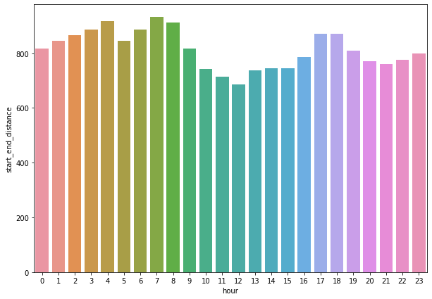
从这个图中,我们可以观察到,距离这个目标特征与小时之间没什么明显的关系或者说规律。
即不同时间段对用户出行并没有什么影响。
距离与车类型
我们知道,初代的摩拜单车比较笨重,很难骑;第二代的摩拜单车比较轻便;
那有没有可能,用户会因为车子轻便,就多骑行一段距离呢?我们来验证一下:
df.groupby('biketype').agg({'start_end_distance': 'mean'})
根据输出的结果,第一代车的骑行平均距离约为807.6米,第二代车的骑行平均距离约为824.6米。
这并不能说明什么问题,算不上是显著的差异。
df.groupby('biketype').size() / df.shape[0]
根据输出的结果,第一代车的骑行占比约为60.56%,第二代车的骑行占比约为39.44%。
这与常规的猜测完全不同,我们认为第二代车轻便,所以第二代车的骑行占比会多,但数据推翻了它。
区块深入探索
以一个7位编码的区块为例,我们考虑一个问题?
每天有多少订单 / 多少不同的用户/ 多少不同的车辆从该区块出发或者到达该区块 ?
采取的思路是:(以出发点为例)
- 按照天数,出发点进行group by
- 每个组计算订单数,用户数(去重),车辆数(去重)
- 通过histogram直方图看数据的分布情况
g1 = df.groupby(['date', 'geohashed_start_loc'])

# unique方法返回不同的值,而nuique方法返回不同值的数量
group_data = g1.agg({'orderid': 'count', 'userid': 'nunique', 'bikeid':'nunique'}).reset_index()

group_data.head()
执行
| date | geohashed_start_loc | orderid | userid | bikeid | |
|---|---|---|---|---|---|
| 0 | 2017-05-10 | wk3n2xc | 1 | 1 | 1 |
| 1 | 2017-05-10 | wk3n80r | 1 | 1 | 1 |
| 2 | 2017-05-10 | wkj19r1 | 1 | 1 | 1 |
| 3 | 2017-05-10 | wm3vz39 | 1 | 1 | 1 |
| 4 | 2017-05-10 | wm3yh9t | 1 | 1 | 1 |
group_data[group_data['orderid'] > 100].head()
执行
| date | geohashed_start_loc | orderid | userid | bikeid | |
|---|---|---|---|---|---|
| 4227 | 2017-05-10 | wx4dqqc | 120 | 118 | 120 |
| 4253 | 2017-05-10 | wx4dqrz | 143 | 135 | 138 |
| 4838 | 2017-05-10 | wx4drzw | 121 | 120 | 110 |
| 4839 | 2017-05-10 | wx4drzx | 116 | 116 | 113 |
| 6489 | 2017-05-10 | wx4dw3u | 121 | 118 | 120 |
以上面表格中第一行数据为例,可理解为在区块 wx4dqqc 内,2017年5月10日,从该区块出发的有120个订单,有118个用户(肯定有用户是骑了两次或两次以上的),有120辆单车。
下面我们通过可视化的方式来展现一下。
sns.distplot(group_data['orderid'])
执行
<matplotlib.axes._subplots.AxesSubplot at 0x1c5922ba90>

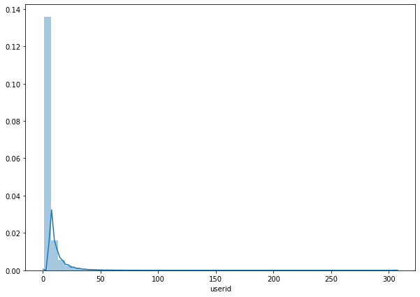
sns.distplot(group_data['userid'])
执行
<matplotlib.axes._subplots.AxesSubplot at 0x1cbeb6f748>
sns.distplot(group_data['bikeid'])
执行
<matplotlib.axes._subplots.AxesSubplot at 0x1ccbfbb400>
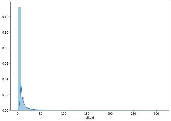
其实从上面三个图中,只能是看出一个大概的分布信息。
具体的数值我们还需要通过 describe 方法来查看。
group_data.describe()
执行
| orderid | userid | bikeid | |
|---|---|---|---|
| count | 631996.000000 | 631996.000000 | 631996.000000 |
| mean | 5.085627 | 4.859236 | 5.041293 |
| std | 8.590106 | 8.313527 | 8.465664 |
| min | 1.000000 | 1.000000 | 1.000000 |
| 25% | 1.000000 | 1.000000 | 1.000000 |
| 50% | 2.000000 | 2.000000 | 2.000000 |
| 75% | 6.000000 | 5.000000 | 6.000000 |
| max | 313.000000 | 307.000000 | 311.000000 |
我们得出结论:平均每天平均每个区块出发的也就是四到五单。同理我们可以计算出平均每天平均每个区块到达的大约在3.5单。毫无疑问这给我们目的地的预测增加了难度。
总和 / 总天数 / 总区块数 = 平均每天平均每个区块 = 总和 / (总天数 * 总区块数) = 总和 / group_data行数
起点终点组合分析
假设根据历史数据,从王府井到天安门的订单较多,那么我们是否可以找到块与块之间的对应,找出topN呢?这显然对于我们出行目的地的预测是有帮助的。
解决思路
- 按照天数,开始区块,结束区块,进行分组
- 每个组计算订单数,用户数,车辆数,进行排序
start_end = df.groupby(['date', 'geohashed_start_loc', 'geohashed_end_loc'])

# 计算每个出发点-停车点 的 订单数,用户数,车辆数,
start_end = start_end.agg({'orderid': 'count', 'userid': 'nunique', 'bikeid': 'nunique', 'start_end_distance': 'mean'}).reset_index().sort_values(by="orderid", ascending=False)

start_end.head()
执行
| date | geohashed_start_loc | geohashed_end_loc | orderid | userid | bikeid | start_end_distance | |
|---|---|---|---|---|---|---|---|
| 318095 | 2017-05-11 | wx4f9ky | wx4f9mk | 71 | 69 | 70 | 385.045143 |
| 1372187 | 2017-05-16 | wx4f9ky | wx4f9mk | 64 | 62 | 64 | 385.045143 |
| 533592 | 2017-05-12 | wx4f9ky | wx4f9mk | 63 | 60 | 62 | 385.045143 |
| 1615438 | 2017-05-18 | wx4f9ky | wx4f9mk | 63 | 63 | 62 | 385.045143 |
| 1143886 | 2017-05-15 | wx4f9ky | wx4f9mk | 62 | 59 | 62 | 385.045143 |
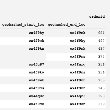
在现有的数据集中,哪个区块到哪个区块的订单数量最多呢?通过以下代码查看
# df.groupby(['geohashed_start_loc', 'geohashed_end_loc']).agg({'orderid': 'count'}).sort_values(by="orderid", ascending=False)[:10]

# 这两行代码输出的结果是等价的
start_end.groupby(['geohashed_start_loc', 'geohashed_end_loc']).agg({'orderid': 'sum'}).sort_values(by="orderid", ascending=False)[:10]
我们获取了Top10的关联,下图是输出的结果
考虑剔除数据
df['geohashed_start_loc_4'] = df['geohashed_start_loc_5'].apply(lambda s: s[:4])
df['geohashed_end_loc_4'] = df['geohashed_end_loc_5'].apply(lambda s: s[:4])

df['geohashed_start_loc_3'] = df['geohashed_start_loc_5'].apply(lambda s: s[:3])
df['geohashed_end_loc_3'] = df['geohashed_end_loc_5'].apply(lambda s: s[:3])

df.head()
执行
| orderid | userid | bikeid | biketype | starttime | geohashed_start_loc | geohashed_end_loc | date | weekday | hour | … | geohashed_start_loc_5 | geohashed_end_loc_5 | start_neighbors_5 | inside_5 | isWeekend | distance | geohashed_start_loc_4 | geohashed_end_loc_4 | geohashed_start_loc_3 | geohashed_end_loc_3 | |
|---|---|---|---|---|---|---|---|---|---|---|---|---|---|---|---|---|---|---|---|---|---|
| 0 | 1893973 | 451147 | 210617 | 2 | 2017-05-14 22:16:50 | wx4snhx | wx4snhj | 2017-05-14 | 周日 | 22 | … | wx4sn | wx4sn | [wx4sj, wx4sp, wx4sm, wx4sq, wx4sr, wx4ev, wx4… | 1 | 1.0 | 384 | wx4s | wx4s | wx4 | wx4 |
| 1 | 4657992 | 1061133 | 465394 | 1 | 2017-05-14 22:16:52 | wx4dr59 | wx4dquz | 2017-05-14 | 周日 | 22 | … | wx4dr | wx4dq | [wx4dq, wx4f2, wx4dw, wx4dx, wx4f8, wx4dn, wx4… | 1 | 1.0 | 798 | wx4d | wx4d | wx4 | wx4 |
| 2 | 2965085 | 549189 | 310572 | 1 | 2017-05-14 22:16:51 | wx4fgur | wx4fu5n | 2017-05-14 | 周日 | 22 | … | wx4fg | wx4fu | [wx4ff, wx4fu, wx4g4, wx4g5, wx4gh, wx4fd, wx4… | 1 | 1.0 | 1120 | wx4f | wx4f | wx4 | wx4 |
| 3 | 4548579 | 489720 | 456688 | 1 | 2017-05-14 22:16:51 | wx4d5r5 | wx4d5r4 | 2017-05-14 | 周日 | 22 | … | wx4d5 | wx4d5 | [wx4d4, wx4dh, wx4d6, wx4d7, wx4dk, wx49f, wx4… | 1 | 1.0 | 117 | wx4d | wx4d | wx4 | wx4 |
| 4 | 3936364 | 467449 | 403224 | 1 | 2017-05-14 22:16:50 | wx4g27p | wx4g266 | 2017-05-14 | 周日 | 22 | … | wx4g2 | wx4g2 | [wx4er, wx4g3, wx4ex, wx4g8, wx4g9, wx4ep, wx4… | 1 | 1.0 | 743 | wx4g | wx4g | wx4 | wx4 |
5 rows × 29 columns
# 出发点和目的地不在同一个g4区块内的
df.loc[df['geohashed_start_loc_4'] != df['geohashed_end_loc_4']].shape[0] / df.shape[0]        # 0.061495985185258936

# 出发点和目的地不在同一个g3区块内的
df.loc[df['geohashed_start_loc_3'] != df['geohashed_end_loc_3']].shape[0] / df.shape[0]        # 0.0006711062768504736
起点和终点不在同一个g4区块内的占比约为 6.15%,不在同一个g3区块内的占比约为 0.06%。
可以考虑直接剔除掉这部分数据了。
模型分析
模型要预测的是用户骑行的终点,为一个geohash的区域,我们可以计算一下整个区域大概有多少。
如果你具备一些基础的分类模型知识,你就会知道要模型分这么多类是不实际的甚至是无法完成的, 因此我们必须做一些规则上的判断。
- 预测模型的GEOHASH4
- 预测模型的GEOHASH5
- 预测模型的GEOHASH6
- 预测模型的GEOHASH7
如果是按照上面这种分层模型来预测,那存在一个很大的弊端,如果第一个geohash4预测错了,那后面的操作就完全无意义了。
做模型的预测时,一定要对数据有一个清晰的认识;如果数据处理不好,那么模型会学习的很糟糕

若有收获,就点个赞吧
0 人点赞
