1.张量
1.1创建张量
张量创建主要有3种方式
- 直接创建
- 依数值创建
- 依概率创建
```python
1.直接创建
a = np.ones((3,3)) arr = torch.tensor(a,device=’cuda’) print(arr)data、dtype
device 所在设备
requires_grad 是否需要梯度
pin_memory 是否锁页内存
2.依据数值创建
a = np.array([[1,2,3],[3,4,5]]) arr = torch.from_numpy(a) print(arr)
通过from_numpy创建的张量适合narrady共享内存的
arr[0][0] = 0 print(a)
创建全零张量 out:输出的张量
out_t = torch.tensor([1]) zero_tensor = torch.zeros((3,3),out=out_t) print(zero_tensor)
创建全一张量 out:输出的张量
out_t = torch.tensor([1]) ones_tensor = torch.ones((3,3),out=out_t) print(ones_tensor)
创建指定数值的全数值张量
full_tensor = torch.full((3,3),10) print(full_tensor)
等差张量
t = torch.arange(1,20,2) print(t)
均分张量
s = torch.linspace(1,20,5) print(s)
对数均分
log = torch.logspace(1,20,5) print(log)
3.依据概率创建
正态分布
根据mean以及std是否为标量还是张量,总共有四种情况
mean1 = torch.arange(1,5,dtype=torch.float) std1 = torch.arange(1,5,dtype=torch.float) guass1 = torch.normal(mean=mean1,std=std1) print(“m张s张:”,guass1) mean0 = 0.0 std0 = 1.0 guass2 = torch.normal(mean=mean0,std=std0,size=(4,1)) print(“m标s标:”,guass2) guass3 = torch.normal(mean=mean1,std=std0) print(“m张s标:”,guass3) guass4 = torch.normal(mean=mean0,std=std1) print(“m标s张:”,guass4)
标准正态分布
stdnol = torch.randn((3,3)) print(stdnol )
均匀分布
r = torch.randint(0,3,(3,3)) print(r)
0~n-1的随即排列
randp = torch.randperm(10) print(randp)
伯努利
b = torch.bernoulli(torch.zeros(3, 3)) print(b)
<a name="DIWih"></a>## 1.2 张量操作操作主要分为3部分:- 拼接与切分- 索引和变形- 压缩与扩展```python# 拼接与切分# torch.cat() 张量序列,dim要拼接维度,在制定维度接续# torch.stack() 张量序列,dim要拼接的维度,在指定维度创建新的张量t = torch.ones((1,3))c1 = torch.cat([t,t,t],dim=0)c2 = torch.cat([t,t,t],dim=1)s1 = torch.stack([t,t,t],dim=0)print(c1,c1.shape)print(c2,c2.shape)print(s1,s1.shape)# 切分# torch.chunk() 将张量按维度平均切分,返回张量列表 chunks要切分的2份数,dim要切分的维度ch1 = torch.chunk(c1,dim=1,chunks=3)ch2 = torch.chunk(c1,dim=0,chunks=3)print(ch1)print(ch2)# torch.split() split_size_or_sections 为int标长度,为list按元素切分list_of_tensor1 = torch.split(t,3,dim=1)list_of_tensor2 = torch.split(t,[1,1,1],dim=1) # list之和等于维度上的长度t[1]print(list_of_tensor1)print(list_of_tensor2)# 索引 torch.index_select\torch.masked_selectt2 = torch.randint(0,9,size=(3,3))print(t2)index = torch.tensor([0,2],dtype=torch.long)idx = torch.index_select(t2,dim=0,index=index) # index的数据类型时指定的必须是torch.longprint(idx)mask = t2.ge(3) # ge大于等于x gt大于x le小于等于 ltms = torch.masked_select(t2,mask) # 通过mask为True进行索引,返回的是一维张量print(ms) # 返回大于等于mask的值# 形状变换torch.reshapet_reshape = torch.reshape(t2,(1,3,3,1))print(t_reshape)# torch.transpose(tensor,dim0=,dim1=) # 交换两个维度# torch.squezze() 压缩# torch.unquezze() 扩展
1.3 张量的数学运算
# 数学运算# 加减除乘torch.add()torch.sub()torch.div()torch.mul()# torch.addcmul() 加法结合乘法# torch.addcdiv() 加法结合除法
1.4 autograd
- autograd.backward() 更新梯度
- autograd.grand() 高阶求导
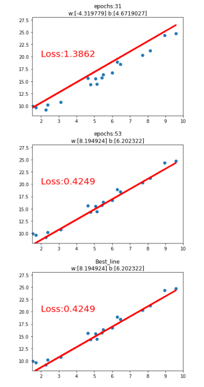
2. 线性回归
import matplotlib.pyplot as pltimport numpy as npimport torch# 线性回归 [y] = [w][x] + [b]best_loss,best_w,best_b = 9999,0,0x = torch.rand(20,1) * 10y = 2*x + (5+torch.randn(20,1))lr = 0.1w = torch.randn((1),requires_grad=True)b = torch.zeros((1),requires_grad=True)for iteration in range(1000):# 前向传播wx = torch.mul(w,x)y_pred = torch.add(wx,b)# loss MSEloss = (0.5 * (y-y_pred)**2).mean()# loss反向传播loss.backward()# 更新参数b.data.sub_(lr * b.grad)w.data.sub_(lr * w.grad)# 作图if loss < best_loss :best_loss,best_w,best_b = loss,w.data.numpy(),b.data.numpy()best_y_pred = y_pred.data.numpy()plt.scatter(x.data.numpy(),y.data.numpy())plt.plot(x.data.numpy(),y_pred.data.numpy(),'r-',lw=3)plt.text(2,20,'Loss:%.4f' % loss.data.numpy(),fontdict={'size':20,'color':'red'})plt.xlim(1.5,10)plt.ylim(8,28)plt.title("epochs:{}\nw:{} b:{}".format(iteration,w.data.numpy(),b.data.numpy()))plt.pause(0.5)if loss.data.numpy()<1:break# 最佳拟合曲线plt.scatter(x.data.numpy(),y.data.numpy())plt.plot(x.data.numpy(),best_y_pred,'r-',lw=3)plt.text(2,20,'Loss:%.4f' % best_loss,fontdict={'size':20,'color':'red'})plt.xlim(1.5,10)plt.ylim(8,28)plt.title("Best_line\nw:{} b:{}".format(best_w,best_b))plt.show()
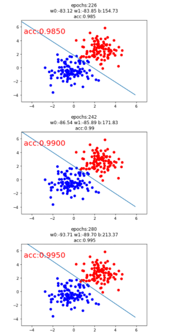
3.逻辑回归
import matplotlib.pyplot as pltimport numpy as npimport torchimport torch.nn as nnsample_num = 100mean_value = 1.5bias = 1n_data = torch.ones(sample_num,2)x0 = torch.normal(mean_value*n_data,1)+biasy0 = torch.zeros(sample_num)x1 = torch.normal(- mean_value*n_data,1)+biasy1 = torch.ones(sample_num)train_x = torch.cat((x0,x1),dim=0)train_y = torch.cat((y0,y1),dim=0)# 超参数lr = 0.01epochs = 100best_acc = -0.1acc=0.0# 逻辑回归模型class LR(nn.Module):def __init__(self):super(LR,self).__init__()self.features = nn.Linear(2,1)self.sigmoid = nn.Sigmoid()def forward(self,x):x = self.features(x)x = self.sigmoid(x)return xpasslr_clf = LR() # 实例化loss_fn = nn.BCELoss()optimizer = torch.optim.SGD(lr_clf.parameters(),lr=lr,momentum=0.9)for iteration in range(1000):# 前向传播y_pred = lr_clf(train_x)# 计算lossloss = loss_fn(y_pred.squeeze(),train_y)# 反向传播loss.backward()# 更新参数optimizer.step()mask = y_pred.ge(0.5).float().squeeze()correct = (mask==train_y).sum()acc = correct.item() / train_y.size(0)# 绘图if best_acc < acc:best_acc = accif best_acc > 0.9:plt.scatter(x0.data.numpy()[:,0],x0.data.numpy()[:,1],c='r',label='class 0')plt.scatter(x1.data.numpy()[:,0],x1.data.numpy()[:,1],c='b',label='class 1')w0,w1 = lr_clf.features.weight[0]w0,w1 = float(w0.item()),float(w1.item())plot_b = float(lr_clf.features.bias[0].item())plot_x = np.arange(-6,6,0.1)plot_y = (- w0 * plot_x - plot_b) / w1plt.xlim(-5,7)plt.ylim(-5,7)plt.plot(plot_x,plot_y)plt.text(-5,5,' acc:%.4f' % best_acc,fontdict={'size':20,'color':'red'})plt.title("epochs:{}\n w0:{:.2f} w1:{:.2f} b:{:.2f} \n acc:{}".format(iteration,w0,w1,plot_b,acc))plt.pause(0.5)if acc >= 0.999:break
4. 数据封装和迭代
- torch.utils.data.DataLoader # 数据迭代器
torch.utils.data.Dataset # 继承类
4.1 Dataset
Dataset是一个继承类,一遍创建一个对象封装好数据读取,实例:
class CustomDataset(data.Dataset):"""下载数据、初始化数据,都可以在这里完成"""# 初始化def __init__(self,data):xy = data # 传入一个numpy数组,最后一列为标签,其余为特征self.x_data = torch.from_numpy(xy[:, 0:-1])self.y_data = torch.from_numpy(xy[:, [-1]])self.len = xy.shape[0]# __getitem_() 主要作用是可以让对象实现迭代功能def __getitem__(self, index):return self.x_data[index], self.y_data[index]# __len__() 主要作用是获取长度def __len__(self):return self.len
4.2 DataLoader
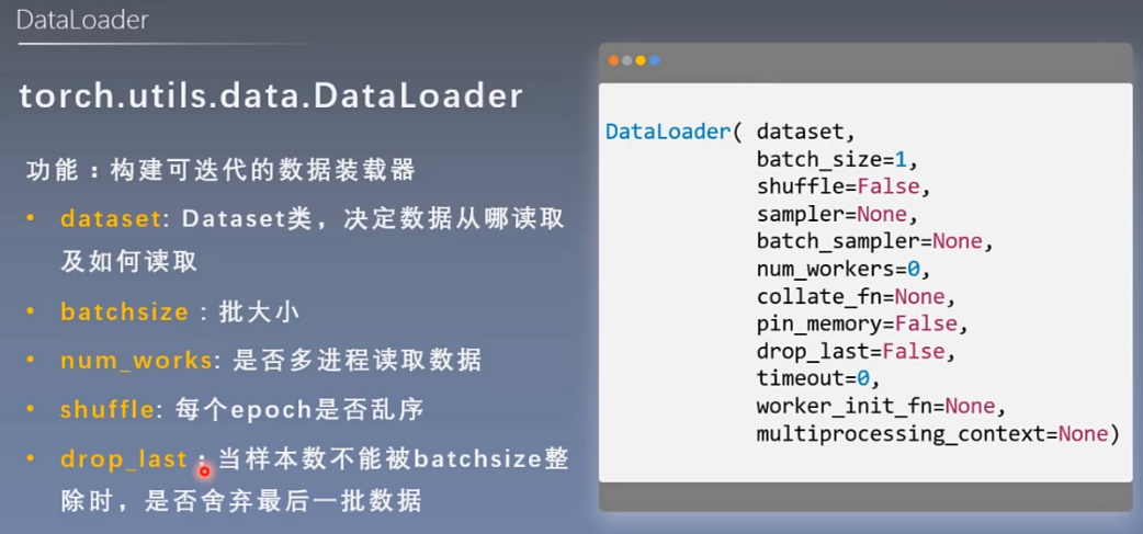
- Epoch:所有训练样本 称为一个Epoch
- iteration:一批数据
- BatchSize:批大小
- 样本总数:80 Batchsize:10 ;1 Epoch = 8 iteration
# 模拟迭代器x = np.random.randint(1,5,(100)).reshape(-1,1)y = np.ones((100),dtype=np.int64).reshape(-1,1)data = np.concatenate((x,y),axis=1)# 实例化数据# 小技巧,添加一个with_labels来区分传入的是带标签还是不带标签的数据train = CustomDataset(data)# 构造迭代器train_loader = DataLoader(dataset=train,batch_size=12,shuffle=True,drop_last=True)# 运行迭代器from torch.autograd import Variablefor epoch in range(2):for i, data in enumerate(train_loader):# 将数据从 train_loader 中读出来,一次读取的样本数是32个inputs, labels = data# 将这些数据转换成Variable类型inputs, labels = Variable(inputs), Variable(labels)# 接下来就是跑模型的环节了,我们这里使用print来代替print("epoch:", epoch, "的第" , i, "个inputs", inputs.data.size(), "labels", labels.data.size())
5.网络模型的创建
建模基本流程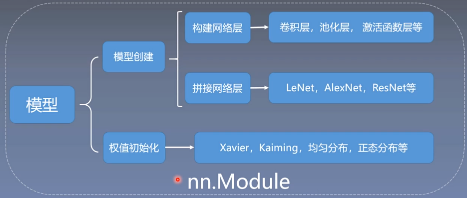
5.1 nn.Module模块
- nn.Parameter 张量子类,表示可学习参数,如weight,bias
- nn.Module 所有网络层基类,管理网络属性
- nn.functional 函数具体实现,如卷积,池化,激活函数等
- nn.init 参数初始化
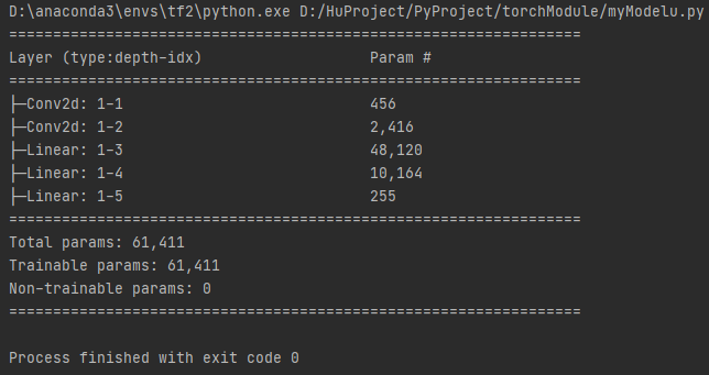
import torch.nn as nnimport torch.nn.functional as Ffrom torchsummary import summaryclass CNNmodel(nn.Module):def __init__(self,classes):super(CNNmodel, self).__init__()self.conv1 = nn.Conv2d(3,6,5)self.conv2 = nn.Conv2d(6,16,5)self.fc1 = nn.Linear(16*5*5,120)self.fc2 = nn.Linear(120,84)self.fc3 = nn.Linear(84,classes)def forward(self,x):out = F.relu(self.conv1(x))out = F.max_pool2d(out,2)out = F.relu(self.conv2(out))out = F.max_pool2d(out,2)# view函数相当于numpy的reshape,-1表示一个不确定的数# 将代码tensor转为一维 和 flatten()类似out = out.view(out.size(0),-1)out = F.relu(self.fc1(out))out = F.relu(self.fc2(out))out = self.fc3(out)return outdef _init_weight(self):for m in self.modules(): # 继承nn.Module的方法if isinstance(m, nn.Conv2d):nn.init.kaiming_normal_(m.weight)elif isinstance(m, nn.BatchNorm2d):m.weight.data.fill_(1)m.bias.data.zero_()# 注意 classes=3 不是 3分类 而是4分类mymodel = CNNmodel(classes=3)mymodel._init_weight()summary(mymodel)
5.2 Containers
- nn.Sequetial 按顺序包装多个网络层 顺序性
- nn.ModuleList 像list一样包装多个网络层 迭代性
- nn.ModuelDict 像dict一样包装多个网络层 索引性
5.2.1 Sequetial
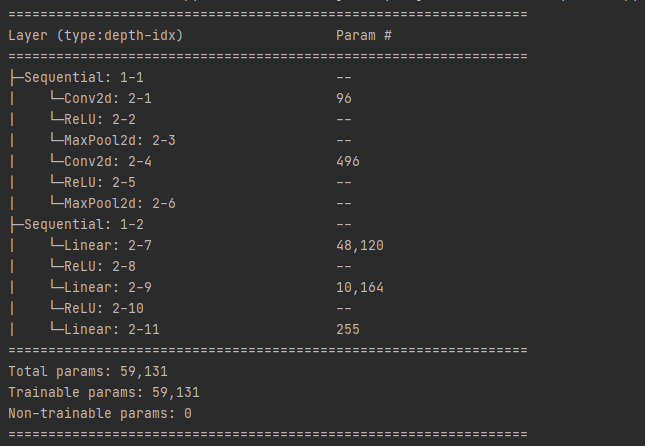
import torch.nn as nnimport torch.nn.functional as Ffrom torchsummary import summaryclass CNNSequential(nn.Module):def __init__(self,classes):super(CNNSequential, self).__init__()# 特征提取self.feature = nn.Sequential(nn.Conv2d(3,6,(5,)),nn.ReLU(),nn.MaxPool2d(kernel_size=2,stride=2),nn.Conv2d(6,16,(5,)),nn.ReLU(),nn.MaxPool2d(kernel_size=2, stride=2),)# 分类self.classifier = nn.Sequential(nn.Linear(16*5*5,120),nn.ReLU(),nn.Linear(120,84),nn.ReLU(),nn.Linear(84,classes))def forward(self,x):out = self.feature(x)out = out.view(out.size[0],-1)out = self.classifier(out)return outdef _init_weight(self):for m in self.modules(): # 继承nn.Module的方法if isinstance(m, nn.Conv2d):nn.init.kaiming_normal_(m.weight)elif isinstance(m, nn.BatchNorm2d):m.weight.data.fill_(1)m.bias.data.zero_()mymodel = CNNSequential(classes=3)mymodel._init_weight()summary(mymodel)
5.2.2 Modules
- append() # 在ModuleList后面添加网络层
- extend() # 拼接两个ModuleList
- insert() # 指定位置传入网络层
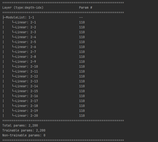
import torchimport torch.nn as nnimport torch.nn.functional as Ffrom torchsummary import summaryclass ModulesList(nn.Module):def __init__(self):super(ModulesList, self).__init__()self.linears = nn.ModuleList([nn.Linear(10,10) for i in range(20)])def forward(self,x):for i,linear in enumerate(self.linears):x = linear(x)return xdef _init_weight(self):for m in self.modules(): # 继承nn.Module的方法if isinstance(m, nn.Conv2d):nn.init.kaiming_normal_(m.weight)elif isinstance(m, nn.BatchNorm2d):m.weight.data.fill_(1)m.bias.data.zero_()# flag2 = Falseflag2 = Trueif flag2:fake_data = torch.ones((10,10))mymodel = ModulesList()mymodel._init_weight()summary(mymodel)output = mymodel(fake_data)print(output)
5.2.3 ModuleDiect
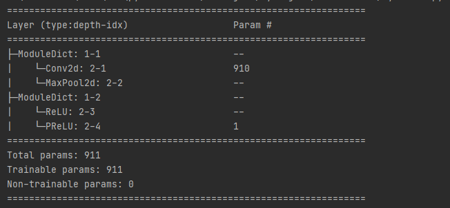
import torchimport torch.nn as nnimport torch.nn.functional as Ffrom torchsummary import summaryclass ModuleDict(nn.Module):def __init__(self):super(ModuleDict, self).__init__()self.choices = nn.ModuleDict({"conv":nn.Conv2d(10,10,3),"pool":nn.MaxPool2d(3),})self.activations = nn.ModuleDict({"relu":nn.ReLU(),"prelu":nn.PReLU(),})def forward(self,x,choice,act):x = self.choices[choice](x)x = self.activations[act](x)return xdef _init_weight(self):for m in self.modules(): # 继承nn.Module的方法if isinstance(m, nn.Conv2d):nn.init.kaiming_normal_(m.weight)elif isinstance(m, nn.BatchNorm2d):m.weight.data.fill_(1)m.bias.data.zero_()# flag3 = Falseflag3 = Trueif flag3:fake_data = torch.randn((4,10,32,32))mymodel = ModuleDict()mymodel._init_weight()summary(mymodel)output = mymodel(fake_data,"conv","prelu")print(output)
6. AlexNet 卷积池化
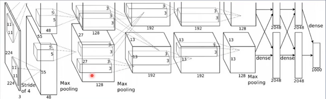
【卷积 - 池化】迭代
#!/usr/bin/env python# -*- encoding: utf-8 -*-'''@File : AlexNet.py@Contact : htkstudy@163.com@Modify Time @Author @Version @Desciption------------ ------- -------- -----------2021/3/29 21:04 Armor(htk) 1.0 None'''import torchimport torch.nn as nnimport torch.nn.functional as Ffrom torchsummary import summaryclass AlexNet(nn.Module):def __init__(self,num_classes=1000):super(AlexNet, self).__init__()self.features = nn.Sequential(nn.Conv2d(3,64,kernel_size=11,stride=4,padding=2),nn.ReLU(inplace=True),nn.MaxPool2d(kernel_size=3,stride=2),nn.Conv2d(64, 192, kernel_size=5, padding=2),nn.ReLU(inplace=True),nn.MaxPool2d(kernel_size=3, stride=2),nn.Conv2d(192, 384, kernel_size=3,padding=1),nn.ReLU(inplace=True),nn.Conv2d(384,256, kernel_size=3, padding=1),nn.ReLU(inplace=True),nn.Conv2d(256,256, kernel_size=3, padding=1),nn.ReLU(inplace=True),nn.MaxPool2d(kernel_size=3,stride=2))self.avgpool = nn.AdaptiveAvgPool2d((6,6))self.classifier = nn.Sequential(nn.Dropout(),nn.Linear(256*6*6,4006),nn.ReLU(inplace=True),nn.Dropout(),nn.Linear(4096,4096),nn.ReLU(inplace=True),nn.Linear(4096,num_classes),)summary(AlexNet())
参数列表
**
Conv2D参数:
- in_channels:输入通道数
- out_channels:输出通道数,等价于卷积核个数
- kernel_size:卷积核大小
- stride:步长
- padding:填充个数
- dilation:空洞卷积大小
- groups:分组卷积设置
- bias:偏置
补充:
- 尺寸计算:……
- ConvTranspose2d 转置卷积
MaxPool2d参数:
- kernel_size:池化核大小
- stride:步长
- padding:填充个数
- dilation:池化核间隔大小
- ceil_mode:尺寸向上取整
- return_indices:记录池化像素索引
AvgPool2d参数:
- kernel_size:池化核大小
- stride:步长
- padding:填充个数
- ceil_mode:尺寸向上取整
- count_include_pad:填充值用于计算
- divisor_override:除法因子
Linear参数:
- in_features:输入结点个数
- out_features:输出结点个数
- bias:偏置
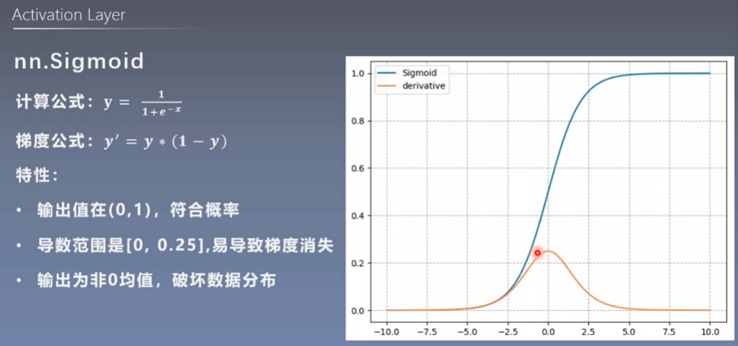
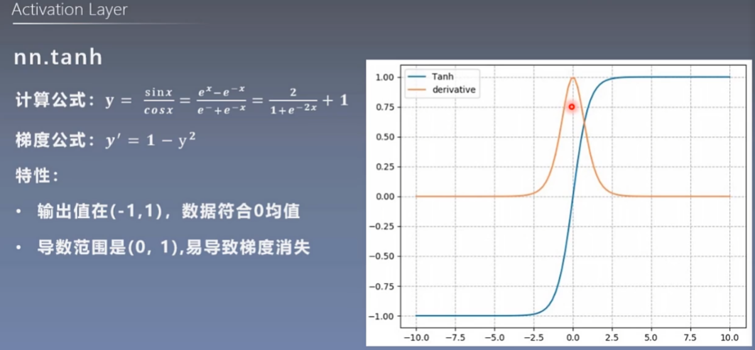
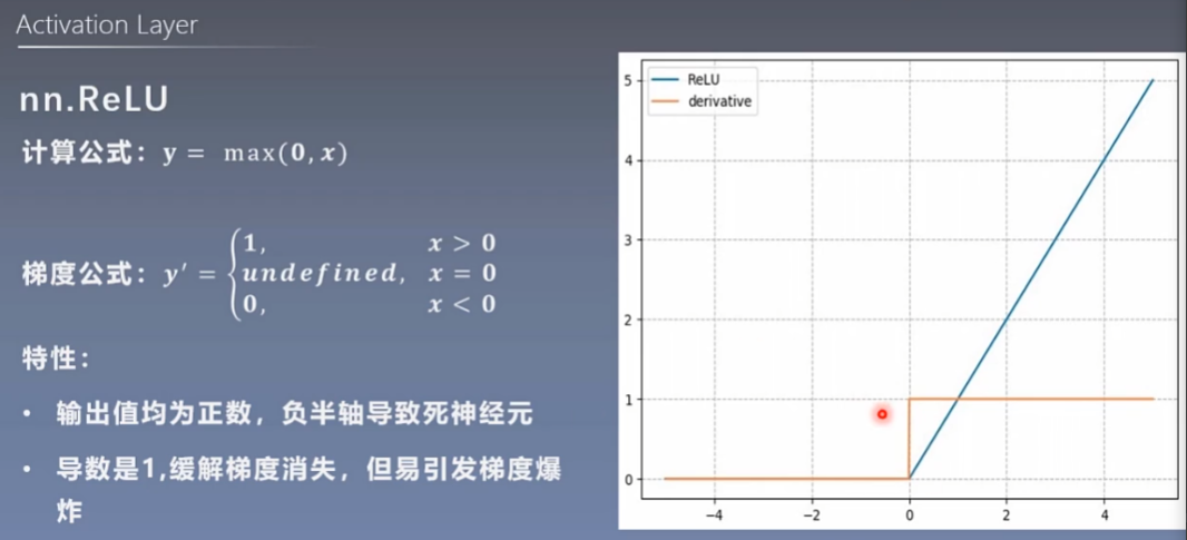
7.激活函数
7.1 nn.Sigmoid
7.2 nn.tanh
7.3 nn.ReLu
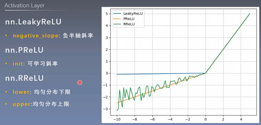
7.4 ReLu变体
- nn.LeakyReLu
- nn.PReLu
- nn.RReLU
8.权值初始化
10种初始化方法
# 初始化nn.init.kaiming_normal_(tensor=m.weight)# 初始化增益nn.init.calculate_gain(nonlinearity='ReLU')
9.损失函数
9.1 nn.CrossEntropyLoss
- 损失函数 Loss Function: 计算一个样本

- 代价函数 Cost Function:计算所有样本的平均值
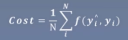
- 目标函数 Object Function:
Obj = Cost + Regularization
交叉熵函数loss_fcuntion = nn.CrossEntropyLoss(weight=,ignore_index=,reduction='mean')
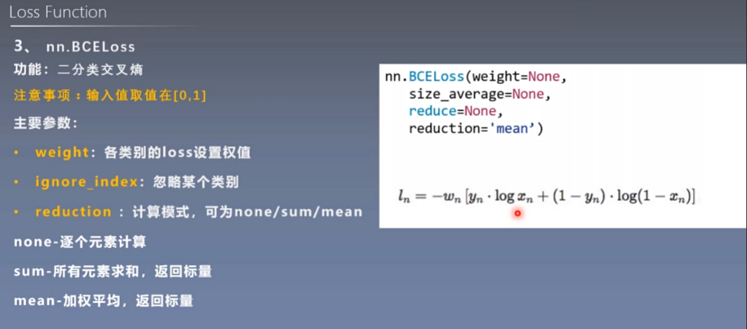
- weight:个类别的loss设置权值
- ignore_index:忽略某个类别
- reduction:计算模式
- mean 加权平均 返回标量
- sum 所有元素求 返回标量
- none 逐个计算
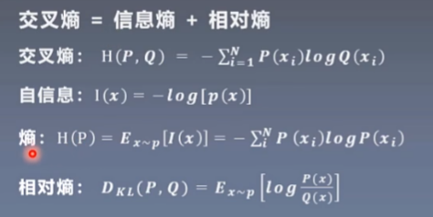
KL散度就是相对熵
# map和lambda结合起来使用,代码更加简洁:list_x = [1, 2, 3, 4, 5, 6, 7, 8]r = map(lambda x:x*x,list_x)print(list(r))-----------------------------------------输出:[1, 4, 9, 16, 25, 36, 49, 64]
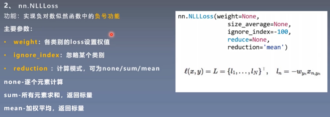
9.2 nn.NLLoss
9.3 nn.BCELoss
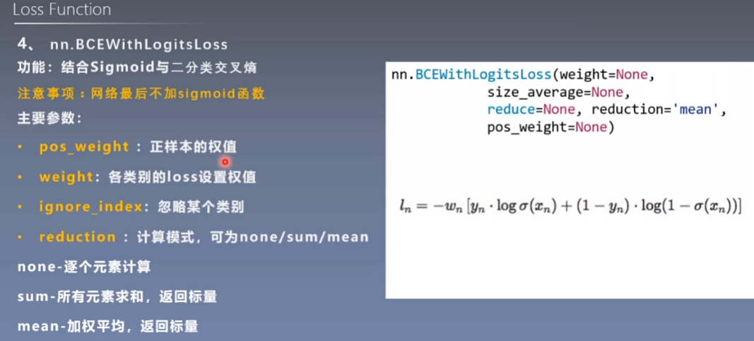
9.4 nn.BCEWithLogitsLoss
9.5 其余14种损失函数
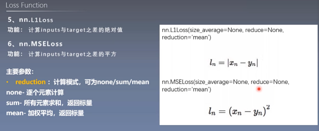
- nn.L1Loss
- nn.MSELoss
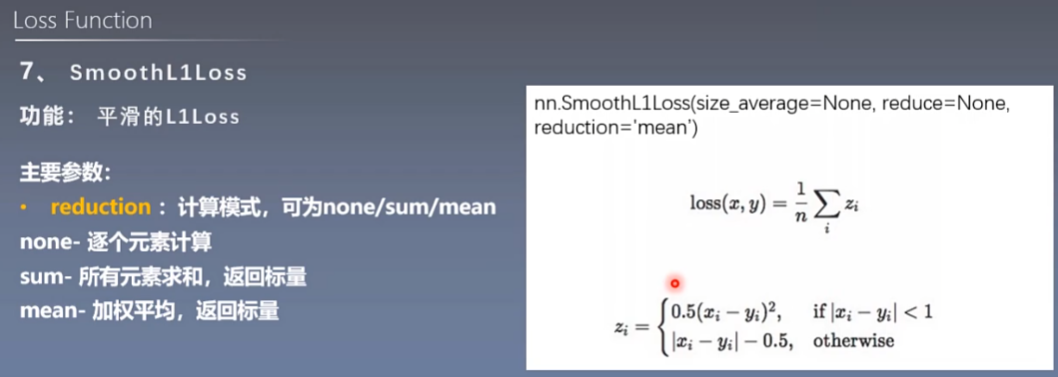
- SmoothL1Loss 平滑
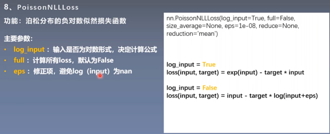
- PoissonNLLLoss 泊松
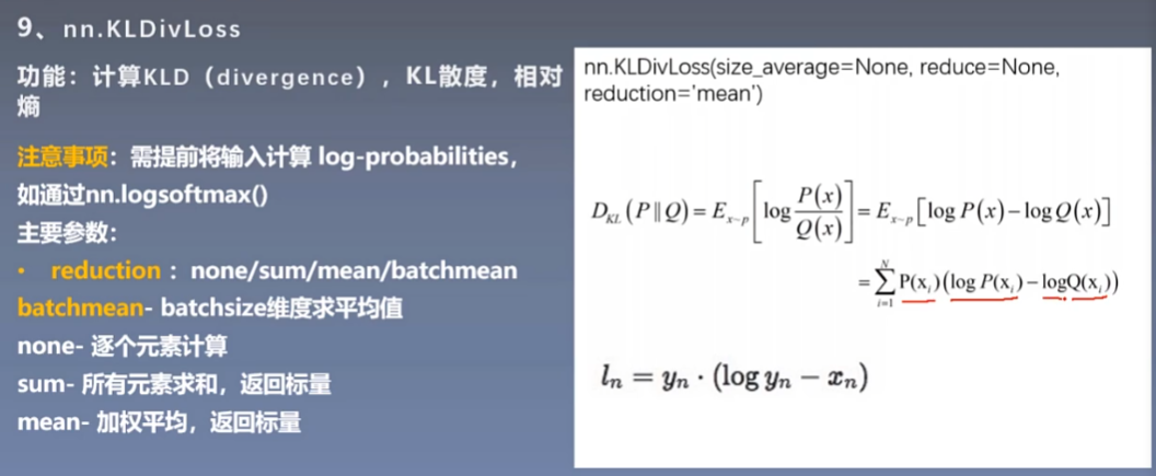
- nn.KLDivLoss KL散度
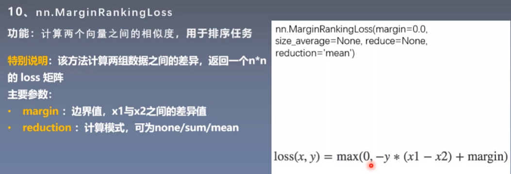
- nn.MarginRankingLoss 排序
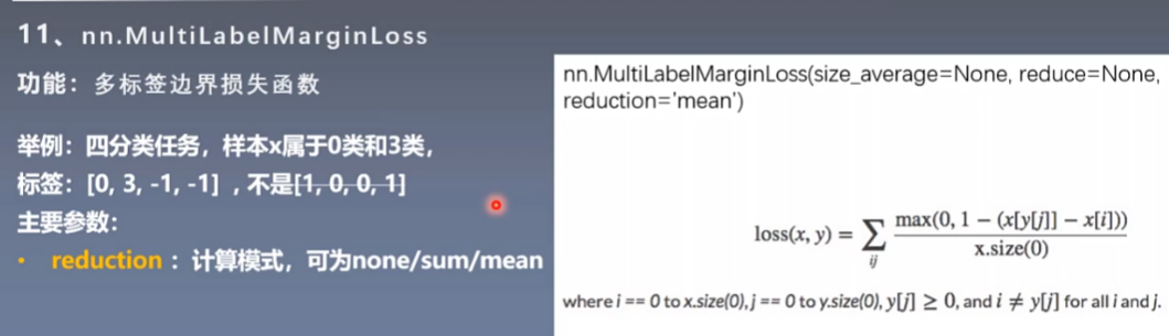
- nn.MultiLabelMarginLoss 多标签
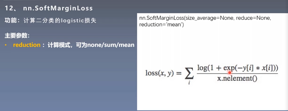
- nn.SoftMarginLoss 二分类
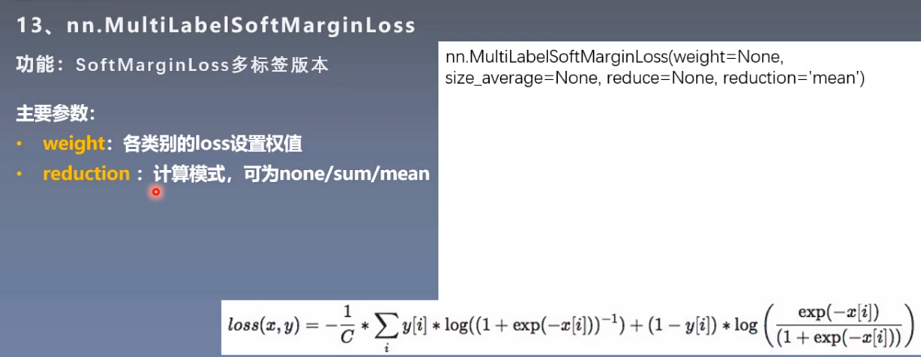
- nn.MultiLabelSoftMarginLoss SoftMarginLoss多标签分类
**
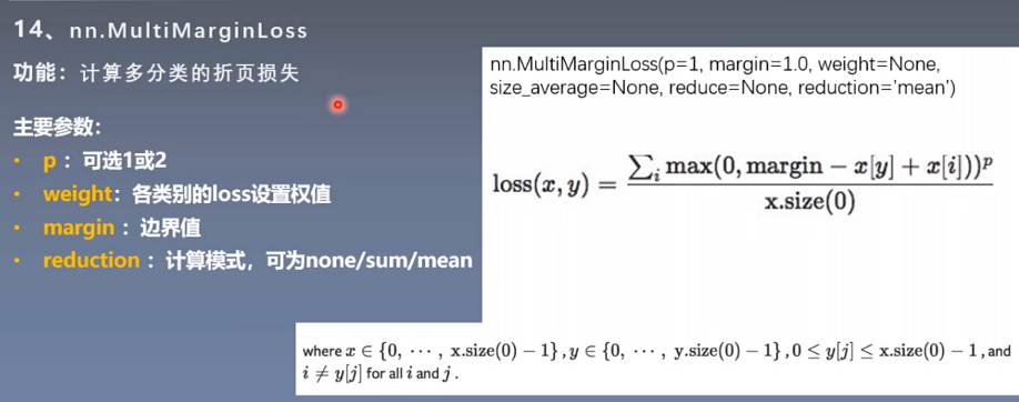
- nn.MultiMarginLoss 多分类
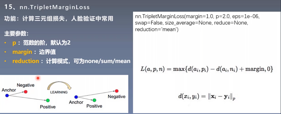
- nn.TripletMarginLoss 三元组损失
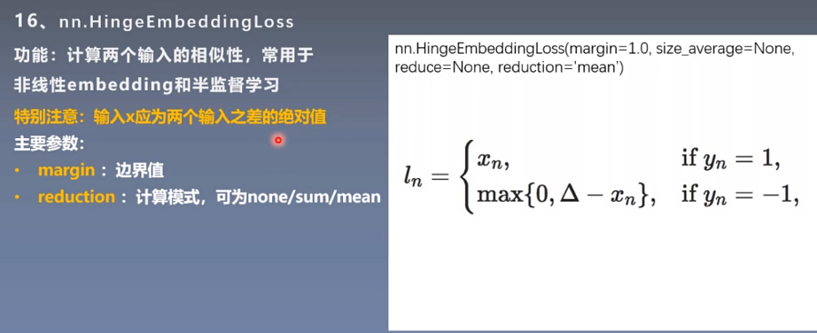
- nn.HingeEmbeddingLoss 非线性相似性损失
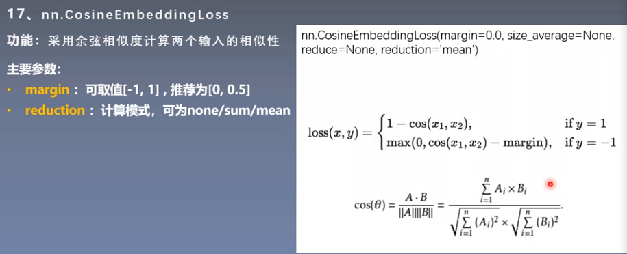
- nn.CosineEmbeddingLoss 余弦相似度 关注方向上的差异
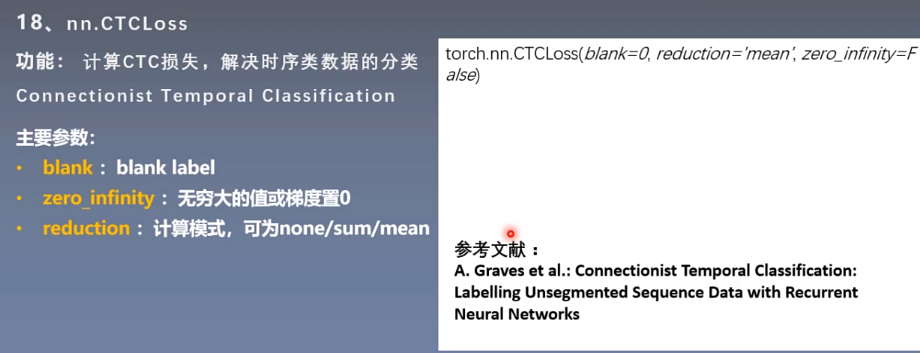
- nn.CTCLoss 时序损失
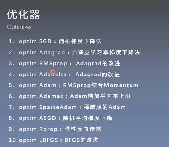
10.优化器
- pytorch特性:张量梯度不自动清零
optim的几个方法
- zero_grad() 清零
- step() 更新
optimizer = nn.optim.Adam()
Momentum 冲量,动量 :结合当前梯度遇上一次更新信息用于当前更新,保持更新惯性。
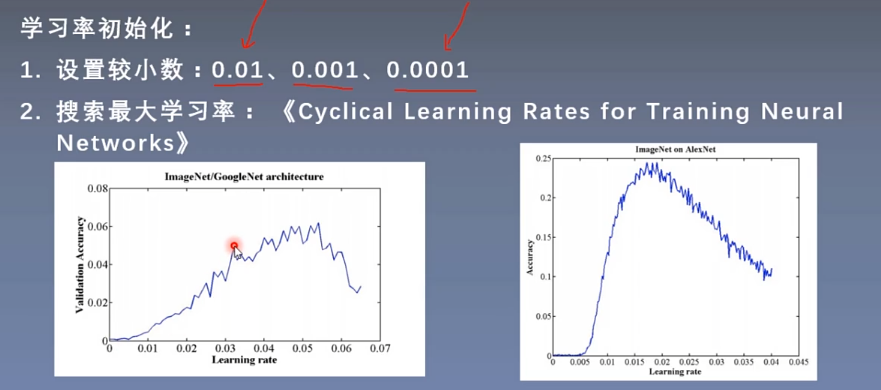
学习率


若有收获,就点个赞吧
0 人点赞
