转载来源:https://github.com/emvolz/treedater
Molecular Clock Dating of Influenza H3N2
Erik Volz
2018-05-02
Introduction
treedater fits a strict or relaxed molecular clock to a phylogenetic tree and estimates evolutionary rates and times of common ancestry. The calendar time of each sample must be specified (possibly with bounds of uncertainty) and the length of the sequences used to estimate the tree.treedater uses heuristic search to optimise the TMRCAs of a phylogeny and the substitution rate. An uncorrelated relaxed molecular clock accounts for rate variation between lineages of the phylogeny which is parameterised using a Gamma-Poisson mixture model.
To cite:
- E.M. Volz and Frost, S.D.W. (2017) Scalable relaxed clock phylogenetic dating. Virus Evolution.
The most basic usage is
dater( tre, sts, s)
where
treis anape::phylophylogeny,stsis a named vector of sample times for each tip intresis the length of the genetic sequences used to estimatetreInvoking treedater from the command line
You can also use treedater from the command line without starting R using thetdclscript:
Note that you may need to modify the first line of the./tdcl -hUsage: ./tdcl [-[-help|h] [<logical>]] [-[-treefn|t] <character>] [-[-samplefn|s] <character>] [-[-sequenceLength|l] <double>] [-[-output|o] [<character>]]-t <file> : file name of tree in newick format-s <file> : should be a comma-separated-value file with sample times in format <taxon-id,sample-time> and no header-l <length> : the integer length of sequences in alignment used to construct the tree-o <file>: name of file for saving output
tdclscript with the correct path toRscriptorlittler.Influenza H3N2 HA
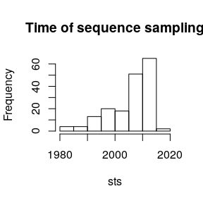
This data set comprises 177 HA sequences collected over 35 years worldwide with known date of sampling. We estimated a maximum likelihood tree using iqtree. We will use the sample dates and ML tree to fit a molecular clock and estimate a dated phylogeny. First, load the tree (any method can be used to load a phylogeny into ape::phylo format):
Note that this tree does not have a root, and in the process of fitting a molecular clock, we will estimate the best root location.require(treedater)#> Loading required package: treedater#> Loading required package: limSolve(tre <- ape::read.tree( system.file( 'extdata', 'flu_h3n2_final_small.treefile', package='treedater') ))#>#> Phylogenetic tree with 177 tips and 175 internal nodes.#>#> Tip labels:#> HM628693_2010-03-03, KC883039_2011-04-04, KC882820_2011-01-04, GQ983548_2009-06-22, KF790184_2012-10-05, JX978746_2012-03-19, ...#>#> Unrooted; includes branch lengths.
To fit the molecular clock, we will need the sample time for each lineage. Note that the date of sampling is incorporated into the name of each lineage, which is common in viral phylogenetics studies. The package includes a convenient function for extracting these dates:seqlen <- 1698 # the length of the HA sequences used to reconstruct the phylogeny
How are samples distributed through time?sts <- sampleYearsFromLabels( tre$tip.label, delimiter='_' )head(sts)#> HM628693_2010-03-03 KC883039_2011-04-04 KC882820_2011-01-04#> 2010.167 2011.255 2011.008#> GQ983548_2009-06-22 KF790184_2012-10-05 JX978746_2012-03-19#> 2009.471 2012.760 2012.213
hist( sts , main = 'Time of sequence sampling')
The basic usage of the treedater algorithm is as follows:
This produces a rooted tree with branches in calendar time. Note that if we invoked(dtr <- dater( tre , sts, seqlen ))#> Note: Minimum temporal branch length (*minblen*) set to 0.0192816582316329. Increase *minblen* in the event of convergence failures.#> Tree is not rooted. Searching for best root position. Increase searchRoot to try harder.#>#> Phylogenetic tree with 177 tips and 176 internal nodes.#>#> Tip labels:#> HM628693_2010-03-03, KC883039_2011-04-04, KC882820_2011-01-04, GQ983548_2009-06-22, KF790184_2012-10-05, JX978746_2012-03-19, ...#>#> Rooted; includes branch lengths.#>#> Time of common ancestor#> 1979.4372056481#>#> Time to common ancestor (before most recent sample)#> 35.6066299683389#>#> Mean substitution rate#> 0.00321644725184376#>#> Strict or relaxed clock#> relaxed#>#> Coefficient of variation of rates#> 0.406223621791838
daterwith a rooted input tree, it would not estimate the root position. In this way, you can also set the root location in other ways, such as by using an outgroup.
Lets see how long it takes to run treedater:
Note the returned value includes estimated substition rates and TMRCAs. Thert0 <- Sys.time()dtr <- dater( tre , sts, seqlen )#> Note: Minimum temporal branch length (*minblen*) set to 0.0192816582316329. Increase *minblen* in the event of convergence failures.#> Tree is not rooted. Searching for best root position. Increase searchRoot to try harder.rt1 <- Sys.time()rt1 - rt0#> Time difference of 2.42605 secs
dtrobject extendsape::phylo, so most of the methods that you can use in other R packages that use that format can also be used with adaterobject. Lets plot the tree.plot( dtr , no.mar=T, cex = .2 )
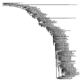
It looks like there are a couple of recent lineages that dont seem to fit well with the ladder-like topology. We will examine this in the next section.Detecting and removing outliers / testing for relaxed clock
To find lineages that dont fit the molecular clock model very well, run
This returns a table in ascending order showing the quality of the molecular clock model fit for each lineage. Now lineages could be selected for removal in various ways. Lets remove all tips that dont have a very high q-value :outliers <- outlierTips( dtr , alpha = 0.20)#> taxon q p loglik#> KF805656_2013-02-21 KF805656_2013-02-21 0.03343122 0.0001888769 -10.256192#> KF805696_2013-02-27 KF805696_2013-02-27 0.12141536 0.0013719249 -7.648289#> KJ955531_2010-08-22 KJ955531_2010-08-22 0.13001919 0.0035424231 -7.123249#> KC883315_2010-11-24 KC883315_2010-11-24 0.13001919 0.0036728583 -6.299932#> CY113269_1980-12-01 CY113269_1980-12-01 0.13001919 0.0032751896 -6.342361#> KP765772_2014-01-01 KP765772_2014-01-01 0.19834490 0.0067235559 -8.163295#> rates branch.length#> KF805656_2013-02-21 0.0005415686 14.6935259#> KF805696_2013-02-27 0.0087076751 0.8178460#> KJ955531_2010-08-22 0.0085105748 1.2451030#> KC883315_2010-11-24 0.0011936366 1.6149868#> CY113269_1980-12-01 0.0071869330 0.4813258#> KP765772_2014-01-01 0.0009823168 33.5660253
Now we can reruntre2 <- ape::drop.tip( tre, rownames(outliers[outliers$q < 0.20,]) )
daterwith the reduced tree:
After removing the outliers, the coefficient of variation of rates is much lower, suggesting that a strict clock model may be appropriate for the reduced tree. We can test the suitability of the strict clock with this test:(dtr2 <- dater(tre2, sts, seqlen, ncpu = 1) ) # increase ncpu to use parallel computing#> Note: Minimum temporal branch length (*minblen*) set to 0.0190819514539775. Increase *minblen* in the event of convergence failures.#> Tree is not rooted. Searching for best root position. Increase searchRoot to try harder.#>#> Phylogenetic tree with 171 tips and 170 internal nodes.#>#> Tip labels:#> HM628693_2010-03-03, KC883039_2011-04-04, KC882820_2011-01-04, GQ983548_2009-06-22, KF790184_2012-10-05, JX978746_2012-03-19, ...#>#> Rooted; includes branch lengths.#>#> Time of common ancestor#> 1981.41140738388#>#> Time to common ancestor (before most recent sample)#> 33.632428232555#>#> Mean substitution rate#> 0.004142128271224#>#> Strict or relaxed clock#> relaxed#>#> Coefficient of variation of rates#> 0.232572609267198
Note that therct <- relaxedClockTest( tre2, sts, seqlen, ncpu = 1 ) # increase ncpu to use parallel computing#> Note: Minimum temporal branch length (*minblen*) set to 0.0190819514539775. Increase *minblen* in the event of convergence failures.#> Tree is not rooted. Searching for best root position. Increase searchRoot to try harder.#> Running in quiet mode. To print progress, set quiet=FALSE.#> NOTE: Running with overrideSearchRoot will speed up execution but may underestimate variance.#> NOTE: Running with overrideTempConstraint will speed up execution but may underestimate variance. Bootstrap tree replicates may have negative branch lengths.#> Note: Minimum temporal branch length (*minblen*) set to 0.0190819514539775. Increase *minblen* in the event of convergence failures.#> Tree is not rooted. Searching for best root position. Increase searchRoot to try harder.#> Best clock model: relaxed#> Null distribution of rate coefficient of variation: 0 0.000422194273826786#> Returning best treedater fit
ncpuoption enabled parallel computing to speed up this test.
This test indicates a relaxed clock. Nevertheless, lets re-fit the model to the reduced tree using a strict clock for comparison:(dtr3 <- dater( tre2, sts, seqlen, strict=TRUE ))#> Note: Minimum temporal branch length (*minblen*) set to 0.0190819514539775. Increase *minblen* in the event of convergence failures.#> Tree is not rooted. Searching for best root position. Increase searchRoot to try harder.#>#> Phylogenetic tree with 171 tips and 170 internal nodes.#>#> Tip labels:#> HM628693_2010-03-03, KC883039_2011-04-04, KC882820_2011-01-04, GQ983548_2009-06-22, KF790184_2012-10-05, JX978746_2012-03-19, ...#>#> Rooted; includes branch lengths.#>#> Time of common ancestor#> 1981.50804415544#>#> Time to common ancestor (before most recent sample)#> 33.5357914609983#>#> Mean substitution rate#> 0.00454744152084714#>#> Strict or relaxed clock#> strict#>#> Coefficient of variation of rates#> 0
plot( dtr3 , no.mar=T, cex = .2 )
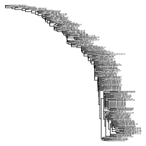
The rate is higher than the initial estimate with the relaxed clock and the recently-sampled outlying lineages have been removed.Parametric bootstrap
Estimating confidence intervals for rates and dates is straightforward using a parametric bootstrap:
How fast was it? Note that thert2 <- Sys.time()(pb <- parboot( dtr3, ncpu = 1) )# increase ncpu to use parallel computing#> Running in quiet mode. To print progress, set quiet=FALSE.#> NOTE: Running with overrideSearchRoot will speed up execution but may underestimate variance.#> NOTE: Running with overrideTempConstraint will speed up execution but may underestimate variance. Bootstrap tree replicates may have negative branch lengths.#> pseudo ML 2.5 % 97.5 %#> Time of common ancestor 1.981508e+03 1.980916e+03 1.981966e+03#> Mean substitution rate 4.547442e-03 4.112521e-03 5.028357e-03#>#> For more detailed output, $trees provides a list of each fit to each simulationrt3 <- Sys.time()
ncpuoption would enable parallel computing.
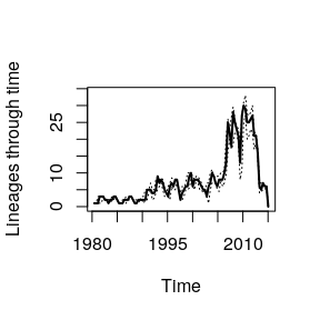
We can also plot the estimated number of lineages through time with confidence intervals:rt3 - rt2#> Time difference of 5.000826 secs
plot( pb )
If the ggplot2 package is installed, we can use that instead:if ( suppressPackageStartupMessages( require(ggplot2)) )(pb.pl <- plot( pb , ggplot=TRUE) )
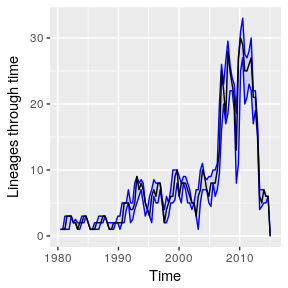
Note repeated bottlenecks and seasonal peaks of LTT corresponding to when samples are taken during seasonal epidemics.
The package also includes methods for nonparametric bootstrapping if you have already computed a bootstrap distribution of phylogenies.Missing sample times
Suppose we only know some of the sample times to the nearest month, a common occurance in viral phylogenetic studies. To simulate this, we will put uncertainty bounds on some sample times equal to a +/- 2-week window. We create the following data frame with columnslowerandupper:
In this case, we constructed the data frame with bounds for the first 50 samples in the tree, but we could also manually construct a data frame for a few selected samples where times of sampling are uncertain, or for all of the samples.sts.df <- data.frame( lower = sts[1:50] - 15/365, upper = sts[1:50] + 15/365 )head(sts.df )#> lower upper#> HM628693_2010-03-03 2010.126 2010.208#> KC883039_2011-04-04 2011.214 2011.296#> KC882820_2011-01-04 2010.967 2011.049#> GQ983548_2009-06-22 2009.430 2009.512#> KF790184_2012-10-05 2012.718 2012.801#> JX978746_2012-03-19 2012.172 2012.254
Now re-run treedater with the uncertain sample times. The vectorstsprovided here gives an initial guess of the unknown sample times.
Note that the estimated rates and dates didnt change very much due to uncertain sample dates in this case.(dtr4 <- dater( tre2, sts, seqlen, strict = TRUE, estimateSampleTimes = sts.df ) )#> Note: Minimum temporal branch length (*minblen*) set to 0.0190819514539775. Increase *minblen* in the event of convergence failures.#> Tree is not rooted. Searching for best root position. Increase searchRoot to try harder.#>#> Phylogenetic tree with 171 tips and 170 internal nodes.#>#> Tip labels:#> HM628693_2010-03-03, KC883039_2011-04-04, KC882820_2011-01-04, GQ983548_2009-06-22, KF790184_2012-10-05, JX978746_2012-03-19, ...#>#> Rooted; includes branch lengths.#>#> Time of common ancestor#> 1981.54481493773#>#> Time to common ancestor (before most recent sample)#> 33.515371994552#>#> Mean substitution rate#> 0.00462062247863572#>#> Strict or relaxed clock#> strict#>#> Coefficient of variation of rates#> 0
(function () { var script = document.createElement(“script”); script.type = “text/javascript”; script.src = “https://mathjax.rstudio.com/latest/MathJax.js?config=TeX-AMS-MML_HTMLorMML“; document.getElementsByTagName(“head”)[0].appendChild(script); })();

