- ggtree: a phylogenetic tree viewer for different types of tree annotations
- Citation
- Introduction
- Getting data into R
- Tree Visualization and Annotation
- Vignette Entry
- Need helps?
- Session info
- References
- —————————————————————————
- Tree Visualization
- Viewing a phylogenetic tree with ggtree
- Layout
- Displaying tree scale (evolution distance)
- Displaying nodes/tips
- Update tree view with a new tree
- Theme
- Visualize a list of trees
- Rescale tree
- Zoom on a portion of tree
- Color tree
- References
- —————————————————————————-
- Tree Manipulation
- Internal node number
- View Clade
- Group Clades
- Group OTUs
- Collapse clade
- Expand collapsed clade
- Scale clade
- Rotate clade
- Flip clade
- Open tree
- Rotate tree
- Interactive tree manipulation
- —————————————————————————
- Tree Annotation
- Annotate clades
- Labelling associated taxa (Monophyletic, Polyphyletic or Paraphyletic)
- Highlight clades
- Taxa connection
- Tree annotation with output from evolution software
- Tree annotation with user specified annotation
- Visualize tree with associated matrix
- Visualize tree with multiple sequence alignment
- Plot tree with associated data
- Plot tree with images and suplots
- References
前言:系统发育树美化R程序包ggtree,由香港大学余光创博士编写。以下内容均为转载,放在这里仅仅为了方便查看。
转载来源:http://127.0.0.1:28433/session/Rvig.368047b416ec.html
参考文献:2041-210X.12628.pdf Ggtree.pdf
余博士其他教程:https://yulab-smu.github.io/treedata-book/chapter5.html?tdsourcetag=s_pcqq_aiomsg
ggtree: a phylogenetic tree viewer for different types of tree annotations
Guangchuang Yu
School of Basic Medical Sciences, Southern Medical University
2019-01-14
- Citation
- Introduction
- Getting data into R
- Tree Visualization and Annotation
- Vignette Entry
- Need helps?
- Session info
- References
You can’t even begin to understand biology, you can’t understand life, unless you understand what it’s all there for, how it arose - and that means evolution. — Richard Dawkins
Citation
If you use ggtree in published research, please cite the most appropriate paper(s) from this list:
- G Yu, DK Smith, H Zhu, Y Guan, TTY Lam. ggtree: an R package for visualization and annotation of phylogenetic trees with their covariates and other associated data. Methods in Ecology and Evolution. 2017, 8(1):28-36. doi: 10.1111/2041-210X.12628.
- G Yu, TTY Lam, H Zhu, Y Guan. Two methods for mapping and visualizing associated data on phylogeny using ggtree. Molecular Biology and Evolution, 2018, 35(2):3041-3043. doi: 10.1093/molbev/msy194.
Introduction
This project arose from our needs to annotate nucleotide substitutions in the phylogenetic tree, and we found that there is no tree visualization software can do this easily. Existing tree viewers are designed for displaying phylogenetic tree, but not annotating it. Although some tree viewers can displaying bootstrap values in the tree, it is hard/impossible to display other information in the tree. Our first solution for displaying nucleotide substituitions in the tree is to add this information in the node/tip names and use traditional tree viewer to show it. We displayed the information in the tree successfully, but we believe this indirect approach is inefficient.
Previously, phylogenetic trees were much smaller. Annotation of phylogenetic trees was not as necessary as nowadays much more data is becomming available. We want to associate our experimental data, for instance antigenic change, with the evolution relationship. Visualizing these associations in a phylogenetic tree can help us to identify evolution patterns. We believe we need a next generation tree viewer that should be programmable and extensible. It can view a phylogenetic tree easily as we did with classical software and support adding annotation data in a layer above the tree. This is the objective of developing the ggtree (Yu et al. 2017). Common tasks of annotating a phylogenetic tree should be easy and complicated tasks can be possible to achieve by adding multiple layers of annotation.
The ggtree is designed by extending the ggplot2 (Wickham 2009) package. It is based on the grammar of graphics and takes all the good parts of ggplot2. There are other R packages that implement tree viewer using ggplot2, including OutbreakTools, phyloseq (McMurdie and Holmes 2013) and ggphylo; they mostly create complex tree view functions for their specific needs. Internally, these packages interpret a phylogenetic as a collection of lines, which makes it hard to annotate diverse user input that are related to node (taxa). The ggtree is different to them by interpreting a tree as a collection of taxa and allowing general flexibilities of annotating phylogenetic tree with diverse types of user inputs.Getting data into R
Most of the tree viewer software (including R packages) focus on Newick and Nexus file format, while there are file formats from different evolution analysis software that contain supporting evidences within the file that are ready for annotating a phylogenetic tree. The treeio package supports several file formats and software outputs. It brings analysis findings to R users for further analysis (e.g. summarization, visualization, comparison and test, etc.). It also allows external data to be mapped on the phylogeny. Please refer to the treeio vignette for more details.
Users can use the following command to open the vignette:
All the data parsed/integrated by treeio package can be used to visualize or annotate phylogenetic tree in ggtree (Yu et al. 2017).vignette("Importer", package="treeio")
Tree Visualization and Annotation
Tree Visualization in ggtree is easy, with one line of commandggtree(tree_object). It supports several layouts, including rectangular, slanted, circular and fan for phylogram and cladogram, equal_angle and daylight for unrooted layout, time-scaled and two dimentional phylogenies. Tree Visualization vignette describes these feature in details.
We implement several functions to manipulate a phylogenetic tree visually, including viewing selected clade to explore large tree, taxa clustering, rotating clade or tree, zoom out or collapsing clades etc..
Tree manipulation functions.
| Function | Descriptiotn |
|---|---|
| collapse | collapse a selecting clade |
| expand | expand collapsed clade |
| flip | exchange position of 2 clades that share a parent node |
| groupClade | grouping clades |
| groupOTU | grouping OTUs by tracing back to most recent common ancestor |
| identify | interactive tree manipulation |
| rotate | rotating a selected clade by 180 degree |
| rotate_tree | rotating circular layout tree by specific angle |
| scaleClade | zoom in or zoom out selecting clade |
| open_tree | convert a tree to fan layout by specific open angle |
Details and examples can be found in Tree Manipulation vignette.
Most of the phylogenetic trees are scaled by evolutionary distance (substitution/site), in ggtree a phylogenetic tree can be re-scaled by any numerical variable inferred by evolutionary analysis ( e.g. species divergence time, d/d, etc). Numerical and category variable can be used to color a phylogenetic tree.
The ggtree package provides several layers to annotate a phylogenetic tree. These layers are building blocks that can be freely combined together to create complex tree visualization.
Geom layers defined in ggtree.
| Layer | Description |
|---|---|
| geom_balance | highlights the two direct descendant clades of an internal node |
| geom_cladelabel | annotate a clade with bar and text label |
| geom_cladelabel2 | annotate a clade with bar and text label for unrooted layout |
| geom_hilight | highlight a clade with rectangle |
| geom_hilight_encircle | highlight a clade with xspline for unrooted layout |
| geom_label2 | modified version of geom_label, with subsetting supported |
| geom_nodelab | layer for node labels, which can be text or image |
| geom_nodepoint | annotate internal nodes with symbolic points |
| geom_point2 | modified version of geom_point, with subsetting supported |
| geom_range | bar layer to present uncertainty of evolutionary inference |
| geom_rootpoint | annotate root node with symbolic point |
| geom_segment2 | modified version of geom_segment, with subsetting supported |
| geom_strip | annotate associated taxa with bar and (optional) text label |
| geom_taxalink | associate two related taxa by linking them with a curve |
| geom_text2 | modified version of geom_text, with subsetting supported |
| geom_tiplab | layer of tip labels, which can be text or image |
| geom_tiplab2 | layer of tip labels for circular layout |
| geom_tippoint | annotate external nodes with symbolic points |
| geom_tree | tree structure layer, with multiple layout supported |
| geom_treescale | tree branch scale legend |
ggtree supports creating phylomoji using Emoji fonts, please refer to the Phylomoji vignette.
ggtree integrates phylopic database and silhouette images of organisms can be downloaded and used to annotate phylogenetic directly. ggtree also supports using local or remote images to annotate a phylogenetic tree. For details, please refer to the ggimage package vignette, which can be opened via the following command:
vignette("ggtree", package="ggimage")
Visualizing an annotated phylogenetic tree with numerical matrix (e.g. genotype table), multiple sequence alignment and subplots are also supported in ggtree. Examples of annotating phylogenetic trees can be found in the Tree Annotation vignette.
Vignette Entry
- Tree Data Import
- Tree Visualization
- Tree Manipulation
- Tree Annotation
- Phylomoji
- Annotating phylogenetic tree with images
- Annotate a phylogenetic tree with insets
ggtree homepage: https://guangchuangyu.github.io/software/ggtree (contains more information about the package, more documentation, a gallery of beautiful published images and links to related resources).
Need helps?
If you have questions/issues, please visit ggtree homepage first. Your problems are mostly documented. If you think you found a bug, please follow the guide and provide a reproducible example to be posted on github issue tracker. For questions, please post to google group. Users are highly recommended to subscribe to the mailing list.
Session info
Here is the output of sessionInfo() on the system on which this document was compiled:
## R version 3.5.2 (2018-12-20)## Platform: x86_64-w64-mingw32/x64 (64-bit)## Running under: Windows Server 2012 R2 x64 (build 9600)#### Matrix products: default#### locale:## [1] LC_COLLATE=C## [2] LC_CTYPE=English_United States.1252## [3] LC_MONETARY=English_United States.1252## [4] LC_NUMERIC=C## [5] LC_TIME=English_United States.1252#### attached base packages:## [1] stats graphics grDevices utils datasets methods base#### loaded via a namespace (and not attached):## [1] compiler_3.5.2 magrittr_1.5 htmltools_0.3.6 tools_3.5.2## [5] prettydoc_0.2.1 yaml_2.2.0 Rcpp_1.0.0 stringi_1.2.4## [9] rmarkdown_1.11 highr_0.7 knitr_1.21 stringr_1.3.1## [13] digest_0.6.18 xfun_0.4 evaluate_0.12
References
McMurdie, Paul J., and Susan Holmes. 2013. “Phyloseq: An R Package for Reproducible Interactive Analysis and Graphics of Microbiome Census Data.” PLoS ONE 8 (4):e61217. https://doi.org/10.1371/journal.pone.0061217.
Wickham, Hadley. 2009. Ggplot2: Elegant Graphics for Data Analysis. 1st ed. Springer.
Yu, Guangchuang, David K. Smith, Huachen Zhu, Yi Guan, and Tommy Tsan-Yuk Lam. 2017. “Ggtree: An R Package for Visualization and Annotation of Phylogenetic Trees with Their Covariates and Other Associated Data.” Methods in Ecology and Evolution 8 (1):28–36. https://doi.org/10.1111/2041-210X.12628.
—————————————————————————
Tree Visualization
Guangchuang Yu and Tommy Tsan-Yuk Lam
School of Basic Medical Sciences, Southern Medical University
2019-01-14
- Viewing a phylogenetic tree with ggtree
- Layout
- Displaying tree scale (evolution distance)
- Displaying nodes/tips
- Update tree view with a new tree
- Theme
- Visualize a list of trees
- Rescale tree
- Zoom on a portion of tree
- Color tree
- References
To view a phylogenetic tree, we first need to parse the tree file into R. The ggtree (Yu et al. 2017) package supports many file formats via the treeio package, including output files of commonly used software packages in evolutionary biology. For more details, plase refer to the treeio vignette.
library("treeio")library("ggtree")nwk <- system.file("extdata", "sample.nwk", package="treeio")tree <- read.tree(nwk)
Viewing a phylogenetic tree with ggtree
The ggtree package extends ggplot2 (Wickham 2009) package to support viewing phylogenetic tree. It implements geom_tree layer for displaying phylogenetic tree, as shown below:
ggplot(tree, aes(x, y)) + geom_tree() + theme_tree()
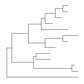
The function, ggtree, was implemented as a short cut to visualize a tree, and it works exactly the same as shown above.
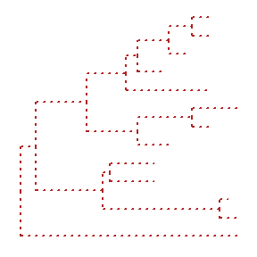
ggtree takes all the advantages of ggplot2. For example, we can change the color, size and type of the lines as we do with ggplot2.
ggtree(tree, color="firebrick", size=1, linetype="dotted")
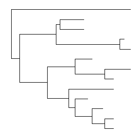
By default, the tree is viewed in ladderize form, user can set the parameter ladderize = FALSE to disable it.
ggtree(tree, ladderize=FALSE)
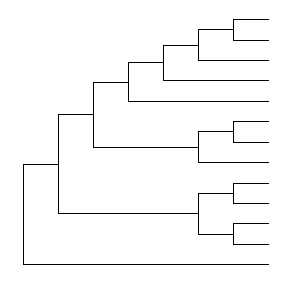
The branch.length is used to scale the edge, user can set the parameter branch.length = “none” to only view the tree topology (cladogram) or other numerical variable to scale the tree (e.g. d/d, see also in Tree Annotation vignette).
ggtree(tree, branch.length="none")
Layout
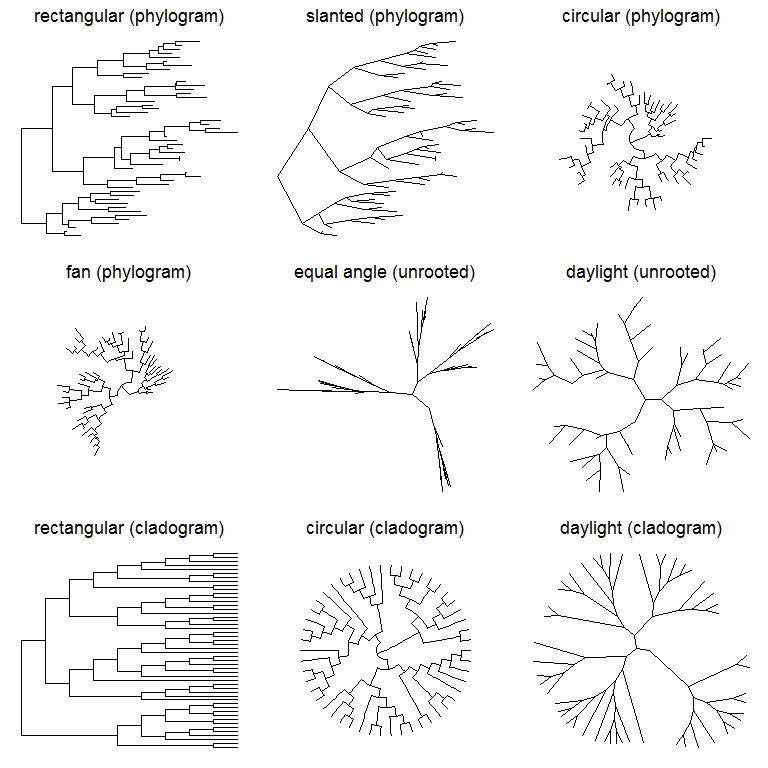
Currently, ggtree supports several layouts, including:
- rectangular (by default)
- slanted
- circular
- fan
for phylogram (by default) and cladogram if user explicitly setting branch.length=‘none’. Unrooted (equal angle and daylight methods), time-scaled and 2-dimensional layouts are also supported.
Phylogram and Cladogram
library(ggtree)set.seed(2017-02-16)tr <- rtree(50)ggtree(tr)ggtree(tr, layout="slanted")ggtree(tr, layout="circular")ggtree(tr, layout="fan", open.angle=120)ggtree(tr, layout="equal_angle")ggtree(tr, layout="daylight")ggtree(tr, branch.length='none')ggtree(tr, branch.length='none', layout='circular')ggtree(tr, layout="daylight", branch.length='none')
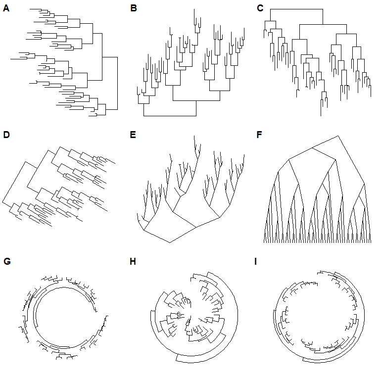
There are also other possible layouts that can be drawn by modifying scales/coordination, for examples, reverse label of time scale, repropotion circular/fan tree, etc..
ggtree(tr) + scale_x_reverse()ggtree(tr) + coord_flip()ggtree(tr) + scale_x_reverse() + coord_flip()print(ggtree(tr), newpage=TRUE, vp=grid::viewport(angle=-30, width=.9, height=.9))ggtree(tr, layout='slanted') + coord_flip()ggtree(tr, layout='slanted', branch.length='none') +coord_flip() + scale_y_reverse() +scale_x_reverse()ggtree(tr, layout='circular') + xlim(-10, NA)ggtree(tr) + scale_x_reverse() + coord_polar(theta='y')ggtree(tr) + scale_x_reverse(limits=c(10, 0)) + coord_polar(theta='y')
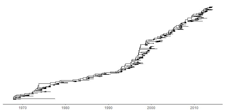
Time-scaled tree
A phylogenetic tree can be scaled by time (time-scaled tree) by specifying the parameter, mrsd (most recent sampling date).
tree2d <- read.beast(system.file("extdata", "twoD.tree", package="treeio"))ggtree(tree2d, mrsd="2014-05-01") + theme_tree2()
Two dimensional tree
ggtree implemented two dimensional tree. It accepts parameter yscale to scale the y-axis based on the selected tree attribute. The attribute should be numerical variable. If it is character/category variable, user should provides a name vector of mapping the variable to numeric by passing it to parameter yscale_mapping.
ggtree(tree2d, mrsd="2014-05-01",yscale="NGS", yscale_mapping=c(N2=2, N3=3, N4=4, N5=5, N6=6, N7=7)) +theme_classic() + theme(axis.line.x=element_line(), axis.line.y=element_line()) +theme(panel.grid.major.x=element_line(color="grey20", linetype="dotted", size=.3),panel.grid.major.y=element_blank()) +scale_y_continuous(labels=paste0("N", 2:7))
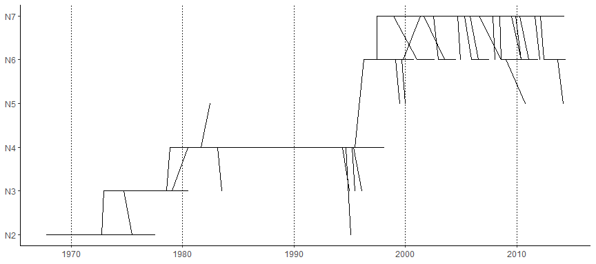
In this example, the figure demonstrates the quantity of y increase along the trunk. User can highlight the trunk with different line size or color using the functions described in Tree Manipulation vignette.
Displaying tree scale (evolution distance)
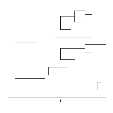
To show tree scale, user can use geom_treescale() layer.
ggtree(tree) + geom_treescale()
geom_treescale() supports the following parameters:
- x and y for tree scale position
- width for the length of the tree scale
- fontsize for the size of the text
- linesize for the size of the line
- offset for relative position of the line and the text
- color for color of the tree scale
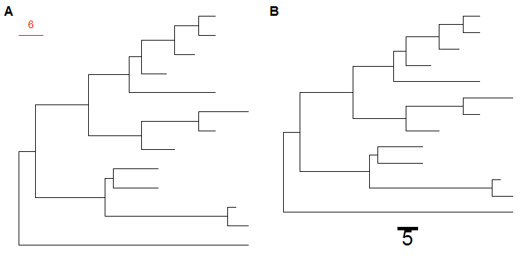
ggtree(tree) + geom_treescale(x=0, y=12, width=6, color='red')ggtree(tree) + geom_treescale(fontsize=8, linesize=2, offset=-1)
We can also usetheme_tree2()to display the tree scale by adding x axis.ggtree(tree) + theme_tree2()
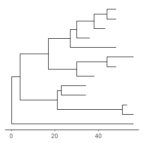
Tree scale is not restricted to evolution distance, ggtree can re-scale the tree with other numerical variable. More details can be found in the Tree Annotation vignette.Displaying nodes/tips
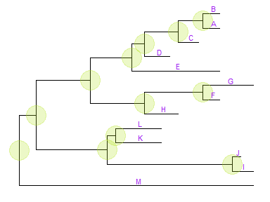
Showing all the internal nodes and tips in the tree can be done by adding a layer of points usinggeom_nodepoint,geom_tippointorgeom_point.ggtree(tree) + geom_point(aes(shape=isTip, color=isTip), size=3)
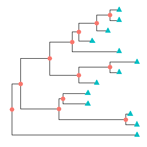
p <- ggtree(tree) + geom_nodepoint(color="#b5e521", alpha=1/4, size=10)p + geom_tippoint(color="#FDAC4F", shape=8, size=3)
Displaying labels
Users can usegeom_textorgeom_labelto display the node (if available) and tip labels simultaneously orgeom_tiplabto only display tip labels:p + geom_tiplab(size=3, color="purple")
geom_tiplabnot only supports using text or label geom to display labels, it also supports image geom to label tip with image files. A corresponding geom,geom_nodelabis also provided for displaying node labels. For details of label nodes with images, please refer to the vignette, Annotating phylogenetic tree with images.
For circular and unrooted layout, ggtree supports rotating node labels according to the angles of the branches.ggtree(tree, layout="circular") + geom_tiplab(aes(angle=angle), color='blue')
To make it more readable for human eye, ggtree provides ageom_tiplab2forcircularlayout (see post 1 and 2).ggtree(tree, layout="circular") + geom_tiplab2(color='blue')
By default, the positions are based on the node positions, we can change them to based on the middle of the branch/edge.p + geom_tiplab(aes(x=branch), size=3, color="purple", vjust=-0.3)
Based on the middle of branch is very useful when annotating transition from parent node to child node.Update tree view with a new tree
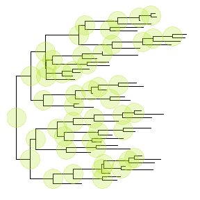
In previous example, we have apobject that stored the tree viewing of 13 tips and internal nodes highlighted with specific colored big dots. If users want to apply this pattern (we can imaging a more complex one) to a new tree, you don’t need to build the tree step by step.ggtreeprovides an operator,%<%, for applying the visualization pattern to a new tree.
For example, the pattern in thepobject will be applied to a new tree with 50 tips as shown below:p %<% rtree(50)
Theme
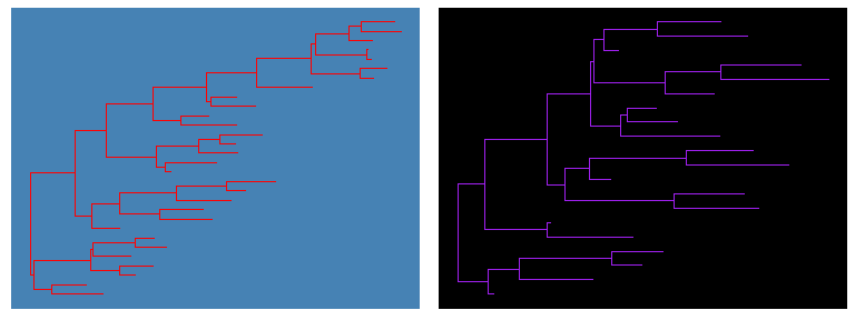
theme_tree()defined a totally blank canvas, whiletheme_tree2()adds phylogenetic distance (via x-axis). These two themes all accept a parameter ofbgcolorthat defined the background color. Users can pass any theme components to thetheme_tree()function to modify them.ggtree(rtree(30), color="red") + theme_tree("steelblue")ggtree(rtree(20), color="white") + theme_tree("black")
Visualize a list of trees
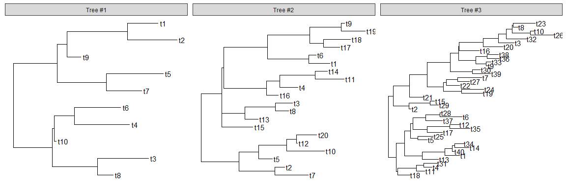
ggtreesupportsmultiPhyloobject and a list of trees can be viewed simultaneously.trees <- lapply(c(10, 20, 40), rtree)class(trees) <- "multiPhylo"ggtree(trees) + facet_wrap(~.id, scale="free") + geom_tiplab()
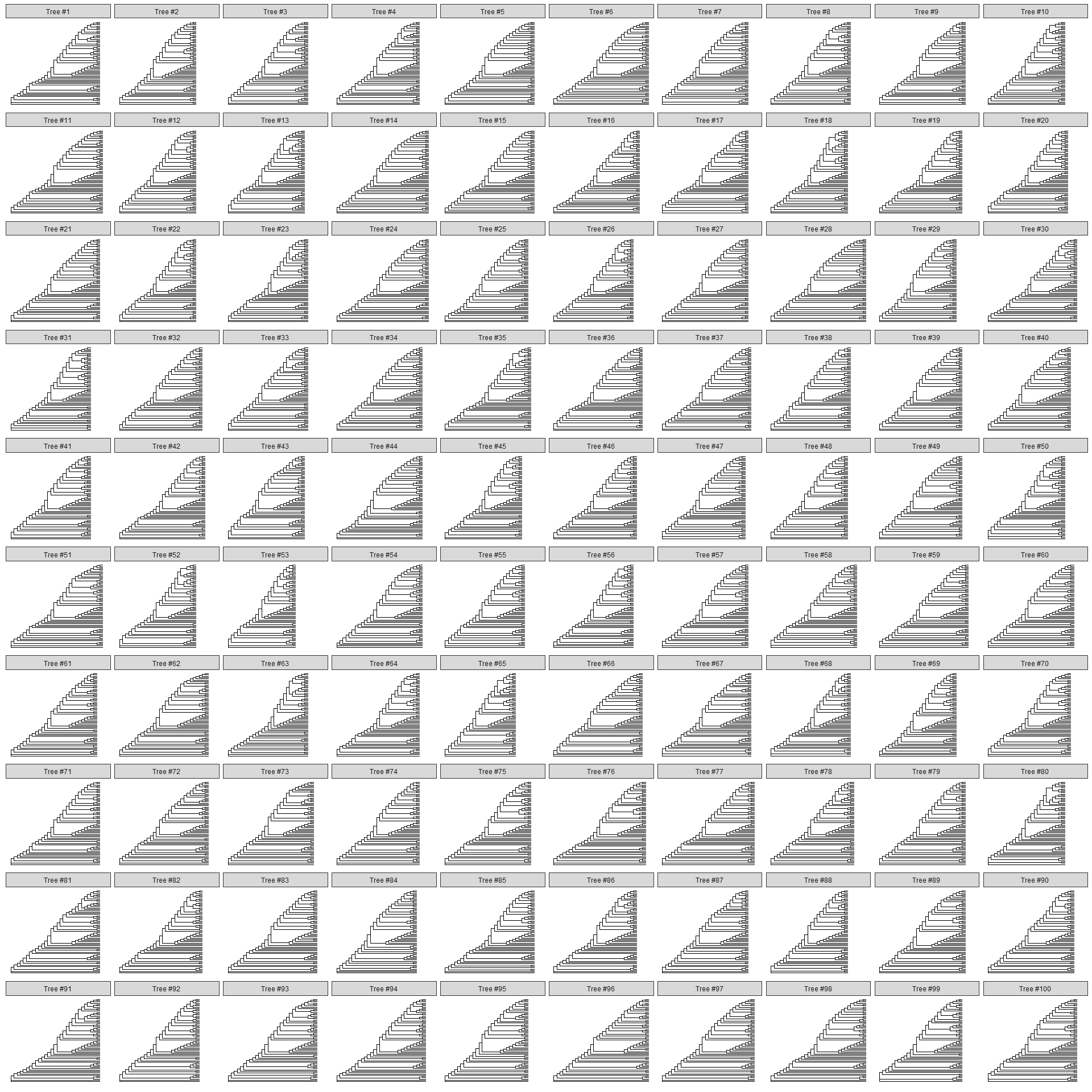
One hundred bootstrap trees can also be view simultaneously.btrees <- read.tree(system.file("extdata/RAxML", "RAxML_bootstrap.H3", package="treeio"))ggtree(btrees) + facet_wrap(~.id, ncol=10)
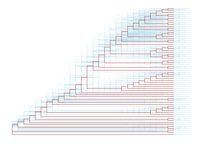
Another way to view the bootstrap trees is to merge them together to form a density tree. We can add a layer of the best tree on the top of the density tree.p <- ggtree(btrees, layout="rectangular", color="lightblue", alpha=.3)best_tree <- read.tree(system.file("extdata/RAxML", "RAxML_bipartitionsBranchLabels.H3", package="treeio"))df <- fortify(best_tree, branch.length='none')p+geom_tree(data=df, color='firebrick')
Rescale tree
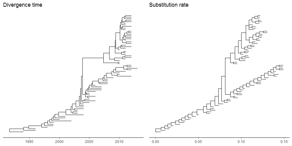
Most of the phylogenetic trees are scaled by evolutionary distance (substitution/site). Inggtree, users can re-scale a phylogenetic tree by any numerical variable inferred by evolutionary analysis (e.g. dN/dS).library("treeio")beast_file <- system.file("examples/MCC_FluA_H3.tree", package="ggtree")beast_tree <- read.beast(beast_file)beast_tree
## 'treedata' S4 object that stored information of## 'C:/Users/biocbuild/bbs-3.8-bioc/tmpdir/RtmpojHSZc/Rinst13901e4f3fa/ggtree/examples/MCC_FluA_H3.tree'.#### ...@ phylo:## Phylogenetic tree with 76 tips and 75 internal nodes.#### Tip labels:## A/Hokkaido/30-1-a/2013, A/New_York/334/2004, A/New_York/463/2005, A/New_York/452/1999, A/New_York/238/2005, A/New_York/523/1998, ...#### Rooted; includes branch lengths.#### with the following features available:## 'height', 'height_0.95_HPD', 'height_median', 'height_range', 'length',## 'length_0.95_HPD', 'length_median', 'length_range', 'posterior', 'rate',## 'rate_0.95_HPD', 'rate_median', 'rate_range'.
p1 <- ggtree(beast_tree, mrsd='2013-01-01') + theme_tree2() +ggtitle("Divergence time")p2 <- ggtree(beast_tree, branch.length='rate') + theme_tree2() +ggtitle("Substitution rate")library(cowplot)plot_grid(p1, p2, ncol=2)
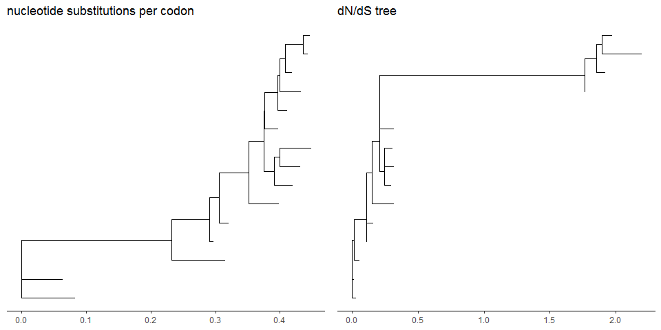
mlcfile <- system.file("extdata/PAML_Codeml", "mlc", package="treeio")mlc_tree <- read.codeml_mlc(mlcfile)p1 <- ggtree(mlc_tree) + theme_tree2() +ggtitle("nucleotide substitutions per codon")p2 <- ggtree(mlc_tree, branch.length='dN_vs_dS') + theme_tree2() +ggtitle("dN/dS tree")plot_grid(p1, p2, ncol=2)
In addition to specifybranch.lengthin tree visualization, users can change branch length stored in tree object by usingrescale_treefunction.beast_tree2 <- rescale_tree(beast_tree, branch.length='rate')ggtree(beast_tree2) + theme_tree2()
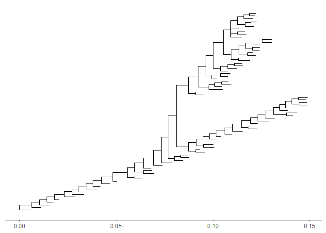
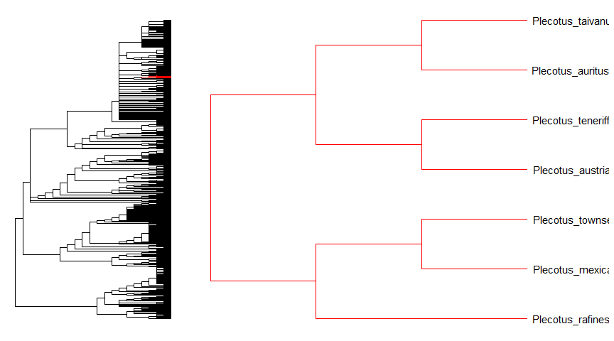
Zoom on a portion of tree
ggtreeprovidesgzoomfunction that similar tozoomfunction provided inape. This function plots simultaneously a whole phylogenetic tree and a portion of it. It aims at exploring very large trees.library("ape")data(chiroptera)library("ggtree")gzoom(chiroptera, grep("Plecotus", chiroptera$tip.label))
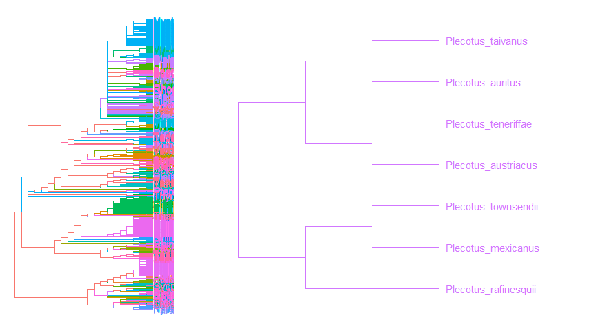
Zoom in selected clade of a tree that was already annotated withggtreeis also supported.groupInfo <- split(chiroptera$tip.label, gsub("_\\w+", "", chiroptera$tip.label))chiroptera <- groupOTU(chiroptera, groupInfo)p <- ggtree(chiroptera, aes(color=group)) + geom_tiplab() + xlim(NA, 23)gzoom(p, grep("Plecotus", chiroptera$tip.label), xmax_adjust=2)
Color tree
Inggtree, coloring phylogenetic tree is easy, by usingaes(color=VAR)to map the color of tree based on a specific variable (numeric and category are both supported).ggtree(beast_tree, aes(color=rate)) +scale_color_continuous(low='darkgreen', high='red') +theme(legend.position="right")
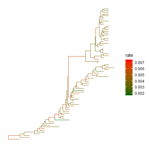
User can use any feature (if available), including clade posterior and dN/dS etc., to scale the color of the tree.References
Wickham, Hadley. 2009. Ggplot2: Elegant Graphics for Data Analysis. 1st ed. Springer.
Yu, Guangchuang, David K. Smith, Huachen Zhu, Yi Guan, and Tommy Tsan-Yuk Lam. 2017. “Ggtree: An R Package for Visualization and Annotation of Phylogenetic Trees with Their Covariates and Other Associated Data.” Methods in Ecology and Evolution 8 (1):28–36. https://doi.org/10.1111/2041-210X.12628.—————————————————————————-
Tree Manipulation
Guangchuang Yu
School of Basic Medical Sciences, Southern Medical University
2019-01-14
- Internal node number
- View Clade
- Group Clades
- Group OTUs
- Collapse clade
- Expand collapsed clade
- Scale clade
- Rotate clade
- Flip clade
- Open tree
- Rotate tree
- Interactive tree manipulation
Internal node number
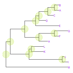
Some of the functions inggtreework with clade and accept a parameter of internal node number. To get the internal node number, user can usegeom_text2to display it:nwk <- system.file("extdata", "sample.nwk", package="treeio")tree <- read.tree(nwk)ggtree(tree) + geom_text2(aes(subset=!isTip, label=node), hjust=-.3) + geom_tiplab()
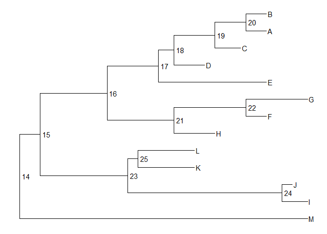
Another way to get the internal node number is usingMRCA()function by providing a vector of taxa names. The function will return node number of input taxa’s most recent commond ancestor (MRCA). It works with tree and graphic object.MRCA(tree, tip=c('A', 'E'))
## [1] 17
MRCA(tree, tip=c('H', 'G'))
## [1] 21
p <- ggtree(tree)MRCA(p, tip=c('A', 'E'))
## [1] 17
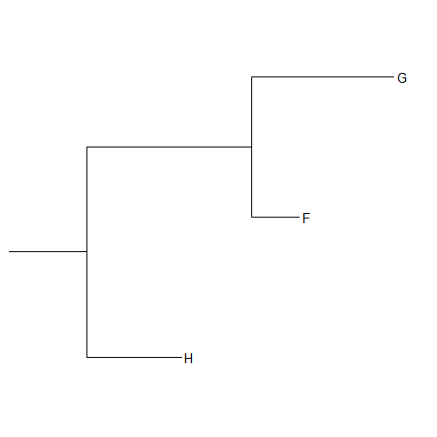
View Clade
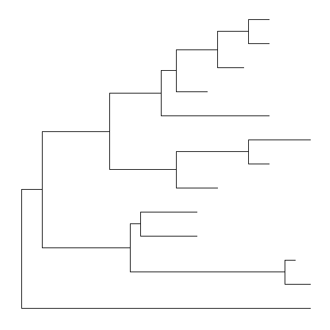
ggtreeprovides a functionviewCladeto visualize a clade of a phylogenetic tree.viewClade(p+geom_tiplab(), node=21)
Group Clades
Theggtreepackage defined several functions to manipulate tree view.groupCladeandgroupOTUmethods were designed for clustering clades or related OTUs.groupCladeaccepts an internal node or a vector of internal nodes to cluster clade/clades.
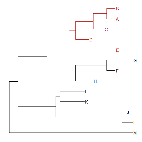
BothgroupCladeandgroupOTUwork fine with tree and graphic object.tree <- groupClade(tree, .node=21)ggtree(tree, aes(color=group, linetype=group))
The following command will produce the same figure.
Withggtree(read.tree(nwk)) %>% groupClade(.node=21) + aes(color=group, linetype=group)
groupCladeandgroupOTU, it’s easy to highlight selected taxa and easy to select taxa to display related features.tree <- groupClade(tree, .node=c(21, 17))ggtree(tree, aes(color=group, linetype=group)) + geom_tiplab(aes(subset=(group==2)))
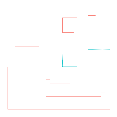
Group OTUs
groupOTUaccepts a vector of OTUs (taxa name) or a list of OTUs.groupOTUwill trace back from OTUs to their most recent common ancestor and cluster them together. Related OTUs are not necessarily within a clade, they can be monophyletic (clade), polyphyletic or paraphyletic.tree <- groupOTU(tree, .node=c("D", "E", "F", "G"))
ggtree(tree, aes(color=group)) + geom_tiplab()
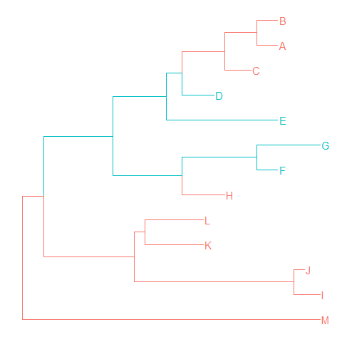
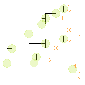
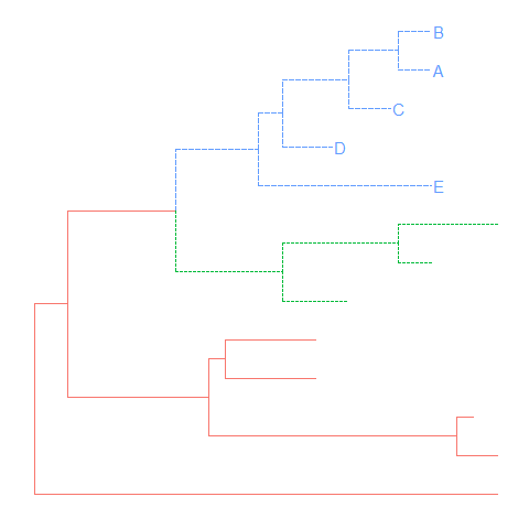
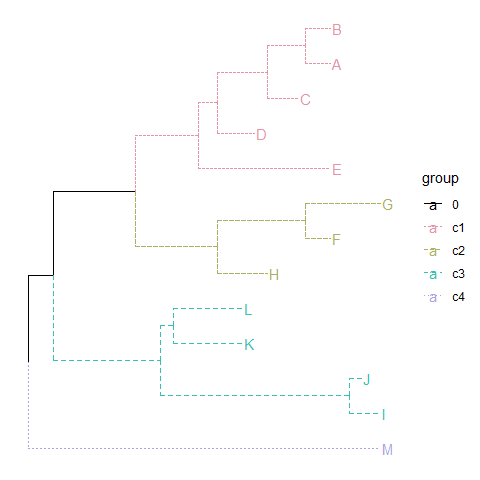
groupOTUcan also input a list of tip groups.cls <- list(c1=c("A", "B", "C", "D", "E"),c2=c("F", "G", "H"),c3=c("L", "K", "I", "J"),c4="M")tree <- groupOTU(tree, cls)library("colorspace")ggtree(tree, aes(color=group, linetype=group)) + geom_tiplab() +scale_color_manual(values=c("black", rainbow_hcl(4))) + theme(legend.position="right")
groupOTUalso works with graphic object.p <- ggtree(tree)groupOTU(p, LETTERS[1:5]) + aes(color=group) + geom_tiplab() + scale_color_manual(values=c("black", "firebrick"))
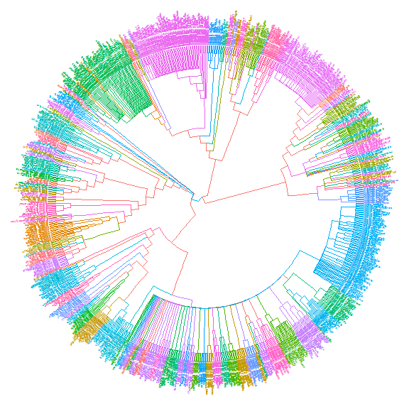
The following example usegroupOTUto display taxa classification.library("ape")data(chiroptera)groupInfo <- split(chiroptera$tip.label, gsub("_\\w+", "", chiroptera$tip.label))chiroptera <- groupOTU(chiroptera, groupInfo)ggtree(chiroptera, aes(color=group), layout='circular') + geom_tiplab(size=1, aes(angle=angle))
Collapse clade
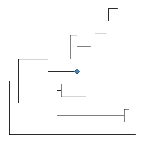
Withcollapsefunction, user can collapse a selected clade.cp <- collapse(p, node=21)cp + geom_point2(aes(subset=(node == 21)), size=5, shape=23, fill="steelblue")
Expand collapsed clade
The collapsed clade can be expanded viaexpandfunction.cp %>% expand(node=21)
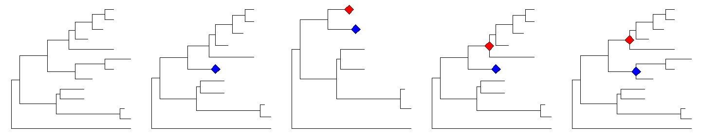
p1 <- ggtree(tree)p2 <- collapse(p1, 21) + geom_point2(aes(subset=(node==21)), size=5, shape=23, fill="blue")p3 <- collapse(p2, 17) + geom_point2(aes(subset=(node==17)), size=5, shape=23, fill="red")p4 <- expand(p3, 17)p5 <- expand(p4, 21)library(cowplot)plot_grid(p1, p2, p3, p4, p5, ncol=5)
Scale clade
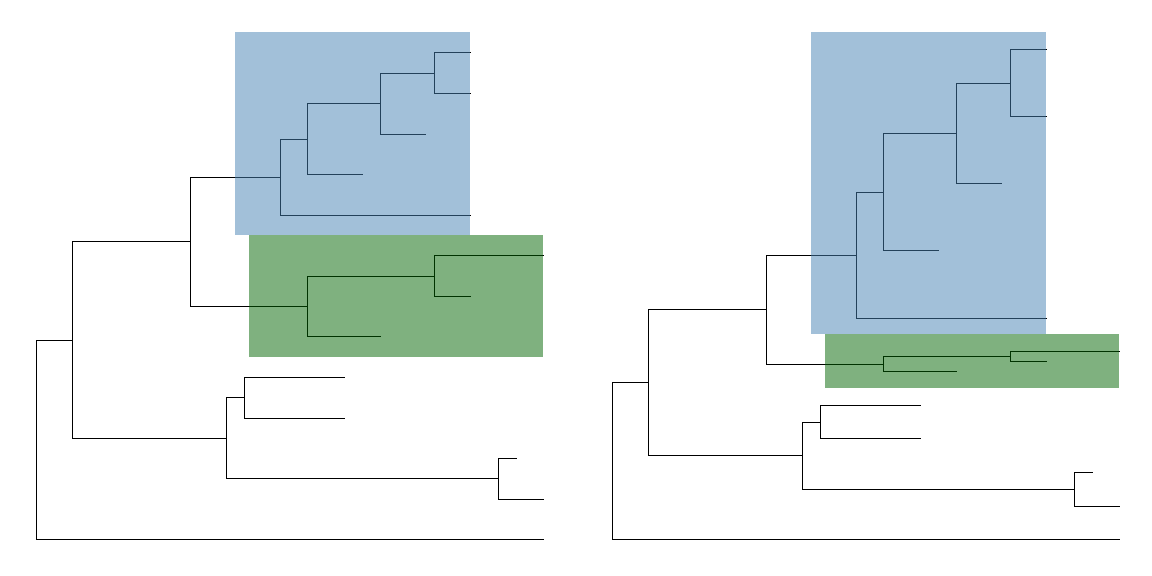
Collpase selected clades can save some space, another approach is to zoom out clade to a small scale.plot_grid(ggtree(tree) + geom_hilight(21, "steelblue"),ggtree(tree) %>% scaleClade(21, scale=0.3) + geom_hilight(21, "steelblue"),ncol=2)
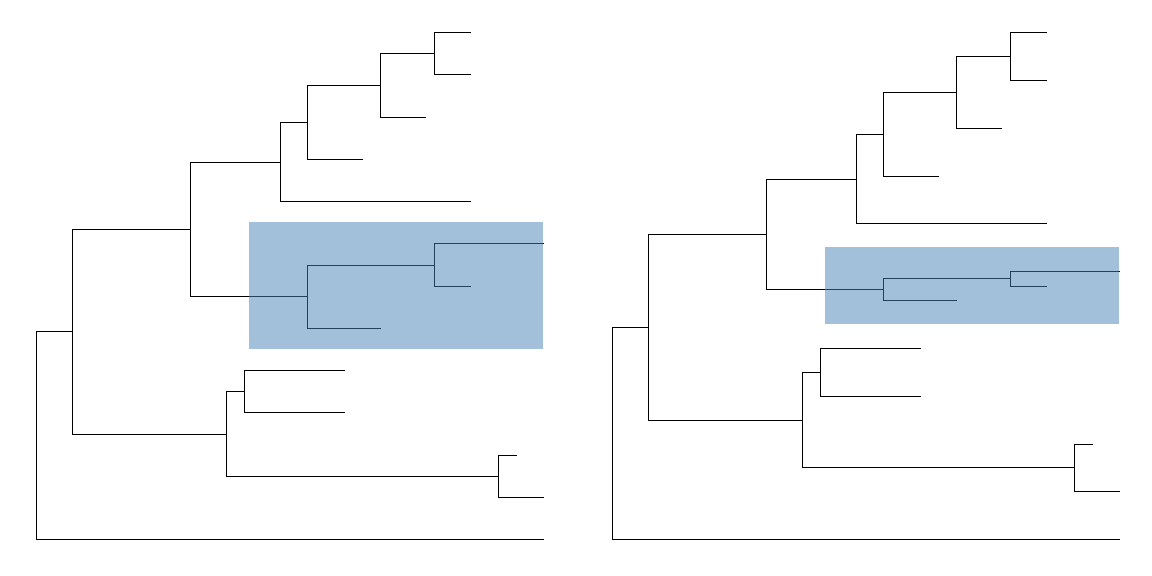
Of course,scaleCladecan acceptscalelarger than 1 and zoom in the selected portion.plot_grid(ggtree(tree) + geom_hilight(17, fill="steelblue") +geom_hilight(21, fill="darkgreen"),ggtree(tree) %>% scaleClade(17, scale=2) %>% scaleClade(21, scale=0.3) +geom_hilight(17, "steelblue") + geom_hilight(21, fill="darkgreen"),ncol=2)
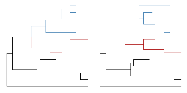
Rotate clade
A selected clade can be rotated by 180 degree usingrotatefunction.tree <- groupClade(tree, c(21, 17))p <- ggtree(tree, aes(color=group)) + scale_color_manual(values=c("black", "firebrick", "steelblue"))p2 <- rotate(p, 21) %>% rotate(17)plot_grid(p, p2, ncol=2)
set.seed(2016-05-29)p <- ggtree(tree <- rtree(50)) + geom_tiplab()for (n in reorder(tree, 'postorder')$edge[,1] %>% unique) {p <- rotate(p, n)print(p + geom_point2(aes(subset=(node == n)), color='red'))}
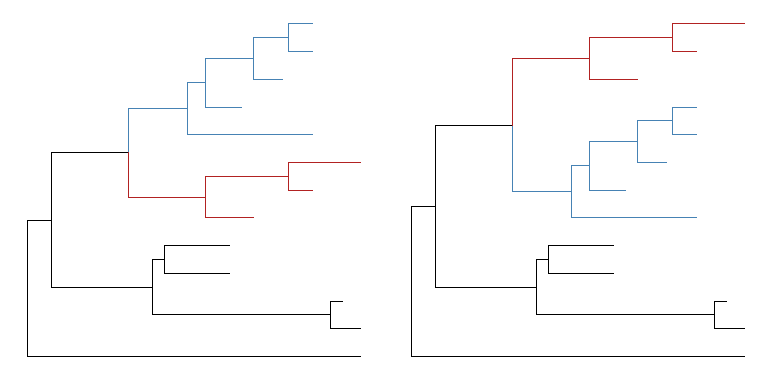
Flip clade
The positions of two selected clades (should share a same parent) can be flip over usingflipfunction.plot_grid(p, flip(p, 17, 21), ncol=2)
Open tree
ggtreesupportsfanlayout and can also transform thecircularlayout tree to afantree by specifying an openangletoopen_treefunction.set.seed(123)tr <- rtree(50)p <- ggtree(tr, layout='circular') + geom_tiplab2()for (angle in seq(0, 270, 10)) {print(open_tree(p, angle=angle) + ggtitle(paste("open angle:", angle)))}

Rotate tree
Rotating acirculartree is supported byrotate_treefunction.for (angle in seq(0, 270, 10)) {print(rotate_tree(p, angle) + ggtitle(paste("rotate angle:", angle)))}
Interactive tree manipulation
Interactive tree manipulation is also possible, please refer to https://guangchuangyu.github.io/2016/06/identify-method-for-ggtree.
—————————————————————————
Tree Annotation
Guangchuang Yu
School of Basic Medical Sciences, Southern Medical University
2019-01-14
- Annotate clades
- Labelling associated taxa (Monophyletic, Polyphyletic or Paraphyletic)
- Highlight clades
- Taxa connection
- Tree annotation with output from evolution software
- Tree annotation with user specified annotation
- Visualize tree with associated matrix
- Visualize tree with multiple sequence alignment
- Plot tree with associated data
- Plot tree with images and suplots
- References
Annotate clades
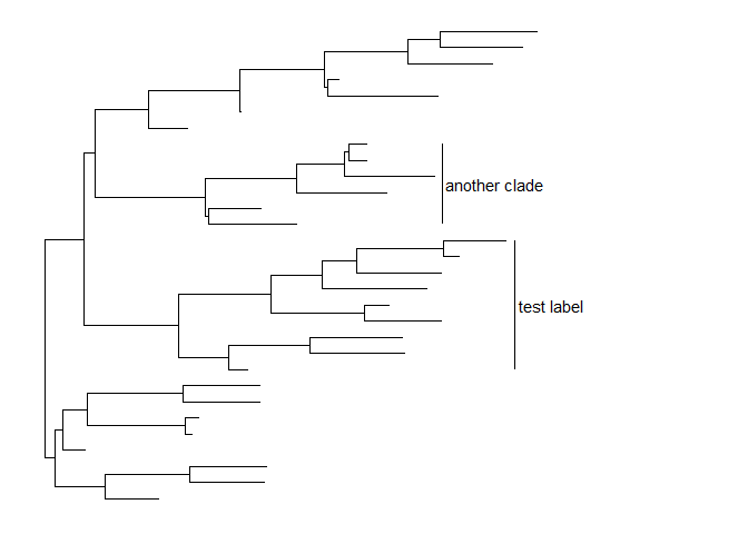
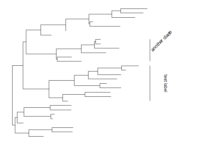
ggtree (Yu et al. 2017) implementsgeom_cladelabellayer to annotate a selected clade with a bar indicating the clade with a corresponding label.
Thegeom_cladelabellayer accepts a selected internal node number. To get the internal node number, please refer to Tree Manipulation vignette.set.seed(2015-12-21)tree <- rtree(30)p <- ggtree(tree) + xlim(NA, 6)p + geom_cladelabel(node=45, label="test label") +geom_cladelabel(node=34, label="another clade")
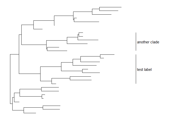
Users can set the parameter,align = TRUE, to align the clade label, and use the parameter,offset, to adjust the position.p + geom_cladelabel(node=45, label="test label", align=TRUE, offset=.5) +geom_cladelabel(node=34, label="another clade", align=TRUE, offset=.5)
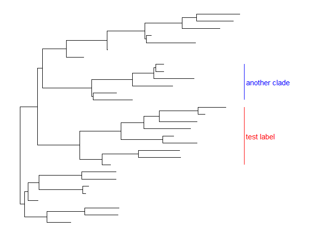
Users can change the color of the clade label via the parametercolor.p + geom_cladelabel(node=45, label="test label", align=T, color='red') +geom_cladelabel(node=34, label="another clade", align=T, color='blue')
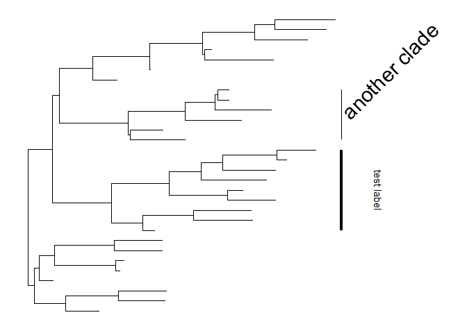
Users can change theangleof the clade label text and relative position from text to bar via the parameteroffset.text.p + geom_cladelabel(node=45, label="test label", align=T, angle=270, hjust='center', offset.text=.5) +geom_cladelabel(node=34, label="another clade", align=T, angle=45)
The size of the bar and text can be changed via the parametersbarsizeandfontsizerespectively.p + geom_cladelabel(node=45, label="test label", align=T, angle=270, hjust='center', offset.text=.5, barsize=1.5) +geom_cladelabel(node=34, label="another clade", align=T, angle=45, fontsize=8)
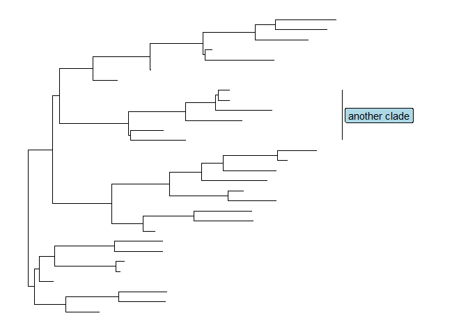
Users can also usegeom_labelto label the text.p + geom_cladelabel(node=34, label="another clade", align=T, geom='label', fill='lightblue')
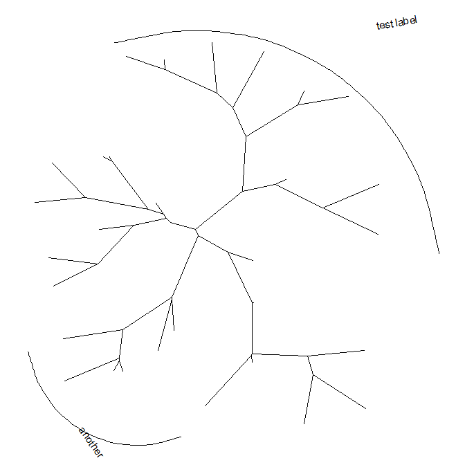
Annotate clades for unrooted tree
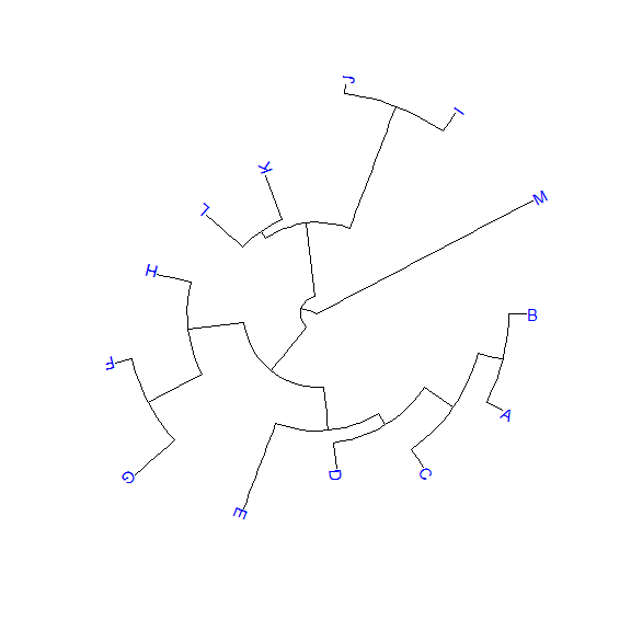
ggtree providesgeom_clade2for labeling clades of unrooted layout trees.pg <- ggtree(tree, layout="daylight")pg + geom_cladelabel2(node=45, label="test label", angle=10) +geom_cladelabel2(node=34, label="another clade", angle=305)
Labelling associated taxa (Monophyletic, Polyphyletic or Paraphyletic)
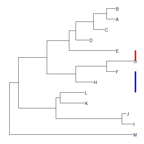
geom_cladelabelis designed for labelling Monophyletic (Clade) while there are related taxa that are not form a clade.ggtreeprovidesgeom_stripto add a strip/bar to indicate the association with optional label (see the issue).nwk <- system.file("extdata", "sample.nwk", package="treeio")tree <- read.tree(nwk)ggtree(tree) + geom_tiplab() +geom_strip(5, 7, barsize=2, color='red') +geom_strip(6, 12, barsize=2, color='blue')
Highlight clades
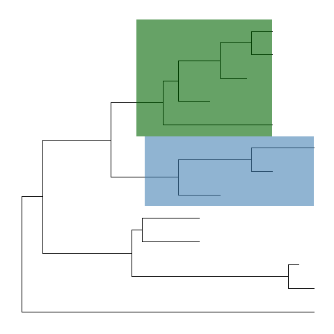
ggtreeimplementsgeom_hilightlayer, that accepts an internal node number and add a layer of rectangle to highlight the selected clade.ggtree(tree) + geom_hilight(node=21, fill="steelblue", alpha=.6) +geom_hilight(node=17, fill="darkgreen", alpha=.6)
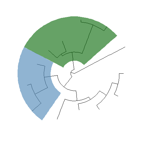
ggtree(tree, layout="circular") + geom_hilight(node=21, fill="steelblue", alpha=.6) +geom_hilight(node=23, fill="darkgreen", alpha=.6)
Another way to highlight selected clades is setting the clades with different colors and/or line types as demonstrated in Tree Manipulation vignette.Highlight balances
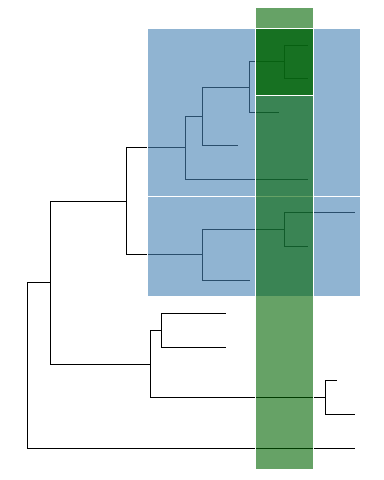
In addition togeom_hilight,ggtreealso implementsgeom_balancewhich is designed to highlight neighboring subclades of a given internal node.ggtree(tree) +geom_balance(node=16, fill='steelblue', color='white', alpha=0.6, extend=1) +geom_balance(node=19, fill='darkgreen', color='white', alpha=0.6, extend=1)
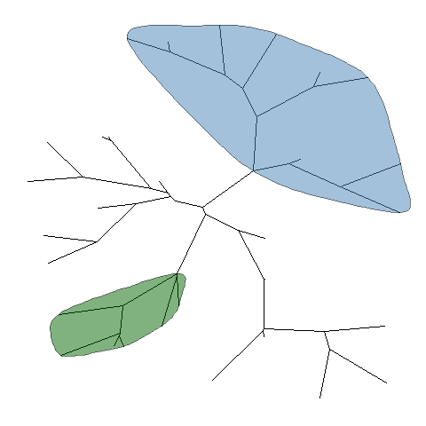
Highlight clades for unrooted tree
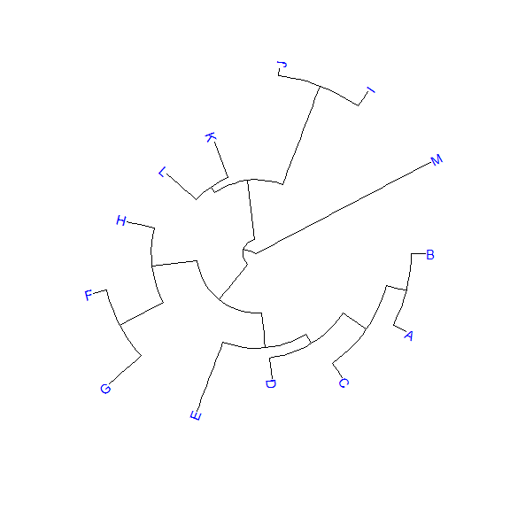
ggtree providesgeom_hilight_encircleto support highlight clades for unrooted layout trees.pg + geom_hilight_encircle(node=45) + geom_hilight_encircle(node=34, fill='darkgreen')
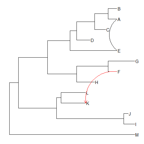
Taxa connection
Some evolutionary events (e.g. reassortment, horizontal gene transfer) can be modeled by a simple tree.ggtreeprovidesgeom_taxalinklayer that allows drawing straight or curved lines between any of two nodes in the tree, allow it to represent evolutionary events by connecting taxa.ggtree(tree) + geom_tiplab() + geom_taxalink('A', 'E') +geom_taxalink('F', 'K', color='red', arrow=grid::arrow(length=grid::unit(0.02, "npc")))
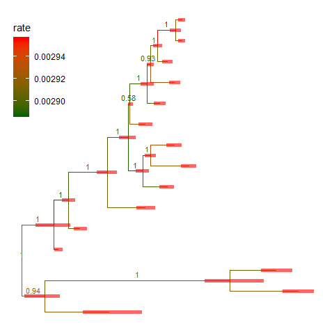
Tree annotation with output from evolution software
The treeio package implemented several parser functions to parse output from commonly used software in evolutionary biology.
Here, we used BEAST (Bouckaert et al. 2014) output as an example. For details, please refer to the Importer vignette.file <- system.file("extdata/BEAST", "beast_mcc.tree", package="treeio")beast <- read.beast(file)ggtree(beast, aes(color=rate)) +geom_range(range='length_0.95_HPD', color='red', alpha=.6, size=2) +geom_nodelab(aes(x=branch, label=round(posterior, 2)), vjust=-.5, size=3) +scale_color_continuous(low="darkgreen", high="red") +theme(legend.position=c(.1, .8))
Tree annotation with user specified annotation
Integrating user data to annotate phylogenetic tree can be done at different levels. The treeio package implementsfull_joinmethods to combine tree data to phylogenetic tree object. The tidytree package supports linking tree data to phylogeny using tidyverse verbs. ggtree supports mapping external data to phylogeny for visualization and annotation on the fly.The
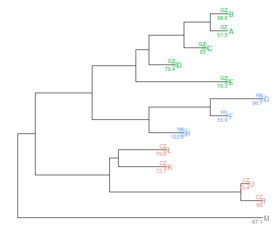
Suppose we have the following data that associate with the tree and would like to attach the data in the tree.%<+%operatornwk <- system.file("extdata", "sample.nwk", package="treeio")tree <- read.tree(nwk)p <- ggtree(tree)dd <- data.frame(taxa = LETTERS[1:13],place = c(rep("GZ", 5), rep("HK", 3), rep("CZ", 4), NA),value = round(abs(rnorm(13, mean=70, sd=10)), digits=1))## you don't need to order the data## data was reshuffled just for demonstrationdd <- dd[sample(1:13, 13), ]row.names(dd) <- NULL
| taxa | place | value | | —- | —- | —- | | D | GZ | 78.4 | | K | CZ | 72.7 | | C | GZ | 83.0 | | H | HK | 102.6 | | E | GZ | 75.3 | | M | NA | 67.1 | | J | CZ | 70.4 | | A | GZ | 51.5 | | B | GZ | 56.6 | | L | CZ | 79.6 | | F | HK | 55.9 | | I | CZ | 68.0 | | G | HK | 86.1 |print(dd)
We can imaging that the place column stores the location that we isolated the species and value column stores numerical values (e.g. bootstrap values).
We have demonstrated using the operator, %<%, to update a tree view with a new tree. Here, we will introduce another operator, %<+%, that attaches annotation data to a tree view. The only requirement of the input data is that its first column should be matched with the node/tip labels of the tree.
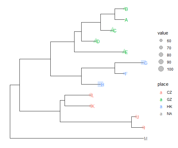
After attaching the annotation data to the tree by %<+%, all the columns in the data are visible to ggtree. As an example, here we attach the above annotation data to the tree view, p, and add a layer that showing the tip labels and colored them by the isolation site stored in place column.
p <- p %<+% dd + geom_tiplab(aes(color=place)) +geom_tippoint(aes(size=value, shape=place, color=place), alpha=0.25)p + theme(legend.position="right")
Once the data was attached, it is always attached. So that we can add other layers to display these information easily.
p + geom_text(aes(color=place, label=place), hjust=1, vjust=-0.4, size=3) +geom_text(aes(color=place, label=value), hjust=1, vjust=1.4, size=3)
Visualize tree with associated matrix
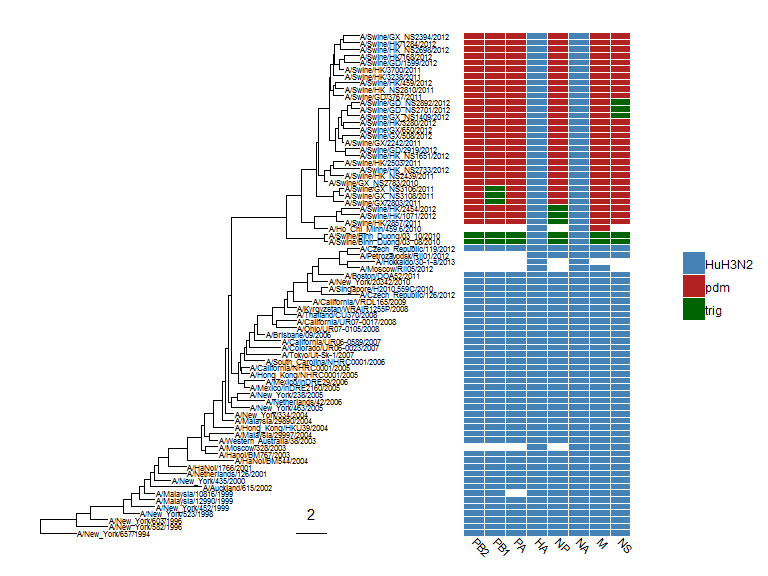
The gheatmap function is designed to visualize phylogenetic tree with heatmap of associated matrix.
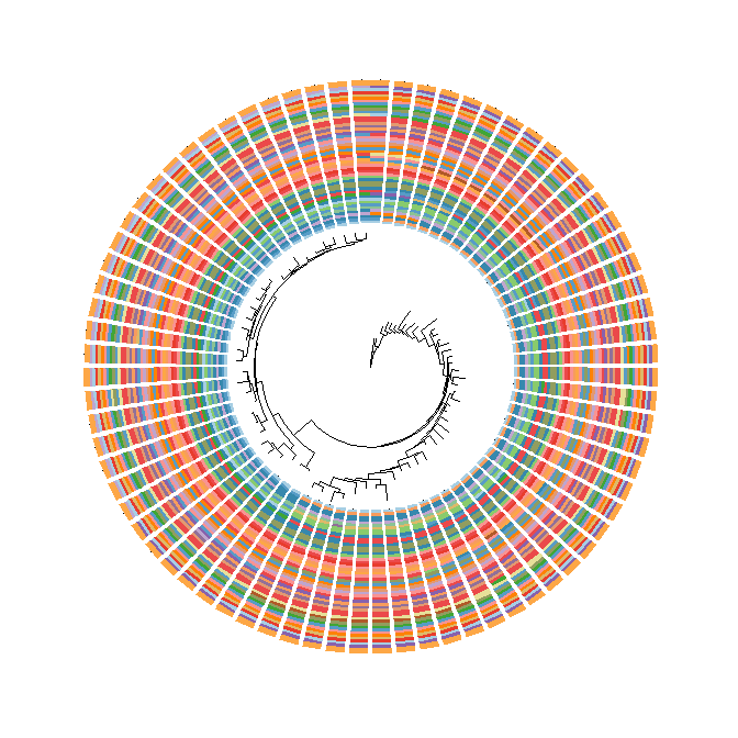
In the following example, we visualized a tree of H3 influenza viruses with their associated genotype.
beast_file <- system.file("examples/MCC_FluA_H3.tree", package="ggtree")beast_tree <- read.beast(beast_file)genotype_file <- system.file("examples/Genotype.txt", package="ggtree")genotype <- read.table(genotype_file, sep="\t", stringsAsFactor=F)colnames(genotype) <- sub("\\.$", "", colnames(genotype))p <- ggtree(beast_tree, mrsd="2013-01-01") + geom_treescale(x=2008, y=1, offset=2)p <- p + geom_tiplab(size=2)gheatmap(p, genotype, offset=5, width=0.5, font.size=3, colnames_angle=-45, hjust=0) +scale_fill_manual(breaks=c("HuH3N2", "pdm", "trig"), values=c("steelblue", "firebrick", "darkgreen"))
The width parameter is to control the width of the heatmap. It supports another parameter offset for controlling the distance between the tree and the heatmap, for instance to allocate space for tip labels.
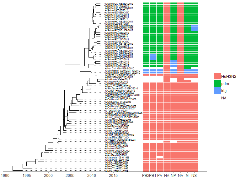
For time-scaled tree, as in this example, it’s more often to use x axis by using theme_tree2. But with this solution, the heatmap is just another layer and will change the x axis. To overcome this issue, we implemented scale_x_ggtree to set the x axis more reasonable.
p <- ggtree(beast_tree, mrsd="2013-01-01") + geom_tiplab(size=2, align=TRUE, linesize=.5) + theme_tree2()pp <- (p + scale_y_continuous(expand=c(0, 0.3))) %>%gheatmap(genotype, offset=8, width=0.6, colnames=FALSE) %>%scale_x_ggtree()pp + theme(legend.position="right")
Visualize tree with multiple sequence alignment
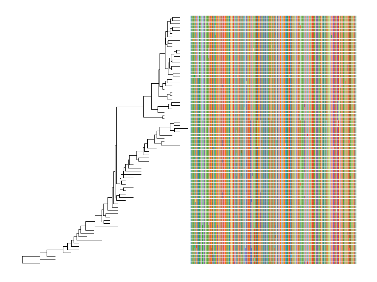
With msaplot function, user can visualize multiple sequence alignment with phylogenetic tree, as demonstrated below:
fasta <- system.file("examples/FluA_H3_AA.fas", package="ggtree")msaplot(ggtree(beast_tree), fasta)
A specific slice of the alignment can also be displayed by specific window parameter.
msaplot(ggtree(beast_tree), fasta, window=c(150, 200)) + coord_polar(theta='y')
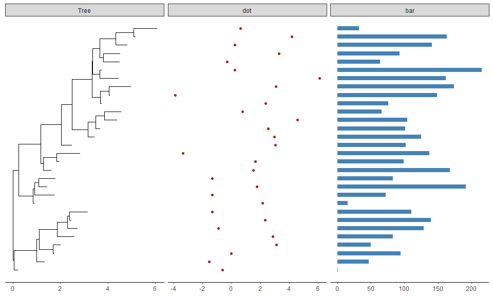
Plot tree with associated data
For associating phylogenetic tree with different type of plot produced by user’s data, ggtree provides facet_plot function which accepts an input data.frame and a geom function to draw the input data. The data will be displayed in an additional panel of the plot.
tr <- rtree(30)d1 <- data.frame(id=tr$tip.label, val=rnorm(30, sd=3))p <- ggtree(tr)p2 <- facet_plot(p, panel="dot", data=d1, geom=geom_point, aes(x=val), color='firebrick')d2 <- data.frame(id=tr$tip.label, value=abs(rnorm(30, mean=100, sd=50)))facet_plot(p2, panel='bar', data=d2, geom=geom_segment, aes(x=0, xend=value, y=y, yend=y), size=3, color='steelblue') + theme_tree2()
Plot tree with images and suplots
Please refer to the following vignettes:
- Annotating phylogenetic tree with images
- Annotate a phylogenetic tree with insets
References
Bouckaert, Remco, Joseph Heled, Denise Kühnert, Tim Vaughan, Chieh-Hsi Wu, Dong Xie, Marc A. Suchard, Andrew Rambaut, and Alexei J. Drummond. 2014. “BEAST 2: A Software Platform for Bayesian Evolutionary Analysis.” PLoS Comput Biol 10 (4):e1003537. https://doi.org/10.1371/journal.pcbi.1003537.
Yu, Guangchuang, David K. Smith, Huachen Zhu, Yi Guan, and Tommy Tsan-Yuk Lam. 2017. “Ggtree: An R Package for Visualization and Annotation of Phylogenetic Trees with Their Covariates and Other Associated Data.” Methods in Ecology and Evolution 8 (1):28–36. https://doi.org/10.1111/2041-210X.12628.

若有收获,就点个赞吧
0 人点赞
