1 应用之数据降噪
1.1 为什么PCA能降噪
在实际的数据中不可避免地出现各种噪音,这些噪音的出现可能会对数据的准确性造成一定的影响。而主成分分析法
还有一个用途就是降噪。PCA通过选取主成分将原有数据映射到低维数据再映射回高维数据的方式进行一定程度的降
噪。
例如,我们构造一组数据
import numpy as npimport matplotlib.pyplot as plt# 造含有噪声的数据X = np.empty((100, 2))X[:, 0] = np.random.uniform(0., 100., size=100)X[:, 1] = 0.75 * X[:, 0] + 3. + np.random.normal(0, 5, size=100)plt.scatter(X[:, 0], X[:, 1])plt.show()
其中np.random.normal(0,5,size=100)就是我们认为添加的噪声,在线性方程上下抖动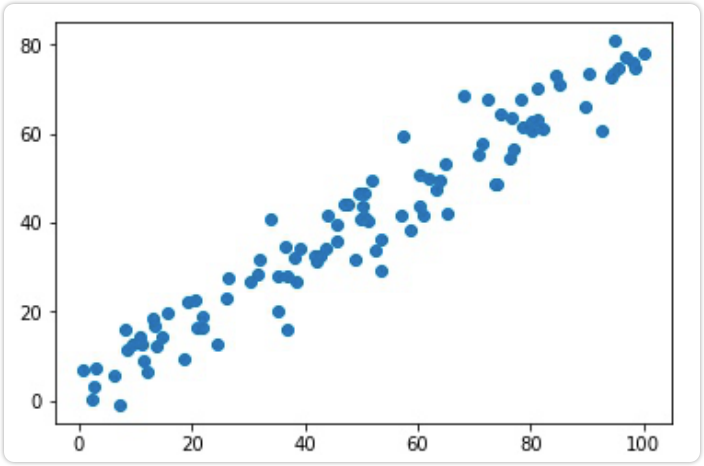
我们降噪,这就需要使用PCA中的一个方法:X_ori=pca.inverse_transform(xpca),将降维后的数据转换成与维度相同数据。要注意,还原后的数据,不等同于原数据!
这是因为在使用PCA降维时,已经丢失了部分的信息(忽略了解释方差比例)。因此在还原时,只能保证维度相同。
会尽最大可能返回原始空间,但不会跟原来的数据一样
这样一来一回之间,丢失掉的信息,就相当于降噪了
在 Stack Overflow中找到了两个不错的答案
- you can only expect this if the number of components you specify is the same as the dimensionality of the input data. For any ncomponents less than this, you will get different numbers than the original dataset after applying the inverse PCA transformation the following diagrams give an illustration in two dimensions
- It can not do that, since by reducing the dimensions with PCA, youve lost information(check pca explainedvarianceratio_for the of information you still have) However it tries its best to go back to the original space as well as it can, see the picture below
对制造的数据先降维,后还原,就可以去除噪音了
# 对含噪声数据先降维,再还原,就实现了降噪from sklearn.decomposition import PCApca = PCA(n_components=1)pca.fit(X)X_reduction = pca.transform(X)X_restore = pca.inverse_transform(X_reduction)plt.scatter(X_restore[:, 0], X_restore[:, 1])plt.show()
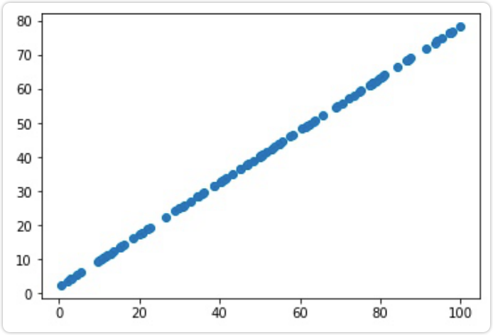
transform降维成一维数据,再 Inverse_ transform返回成二维数据。此时数据成为了一条直线。这个过程可以理解为 降原有的噪音去除了。
当然,我们丢失的信息也不全都是噪音。我们可以将PCA的活成定义为
降低了维度,丢失了信息,也去除了一部分噪音。
**
1.2 手写数字降噪实例
重新创建一个有噪音的数据集,以 digits数据为例
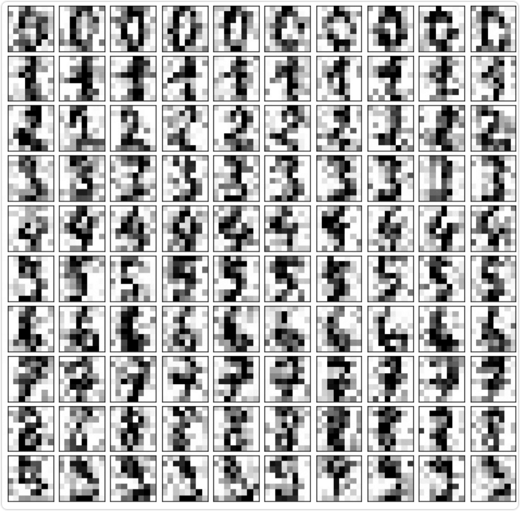
from sklearn import datasetsdigits = datasets.load_digits()X = digits.datay = digits.target# 添加一个正态分布的噪音矩阵noisy_digits = X + np.random.normal(0, 4, size=X.shape)# 绘制噪音数据:从y==0数字中取10个,进行10次循环;# 依次从y=num再取出10个,将其与原来的样本拼在一起example_digits = noisy_digits[y == 0, :][:10]for num in range(1, 10):example_digits = np.vstack([example_digits, noisy_digits[y == num, :][:10]])print(example_digits.shape) # (100, 64)
下面将这100个数字绘制出来,得到有噪音的数字
# 绘制100个数字def plot_digits(data):fig, axes = plt.subplots(10, 10, figsize=(10, 10),subplot_kw={'xticks': [], 'yticks': []},gridspec_kw=dict(hspace=0.1, wspace=0.1))for i, ax in enumerate(axes.flat):ax.imshow(data[i].reshape(8, 8),cmap='binary', interpolation='nearest', clim=(0, 16))plt.show()plot_digits(example_digits)
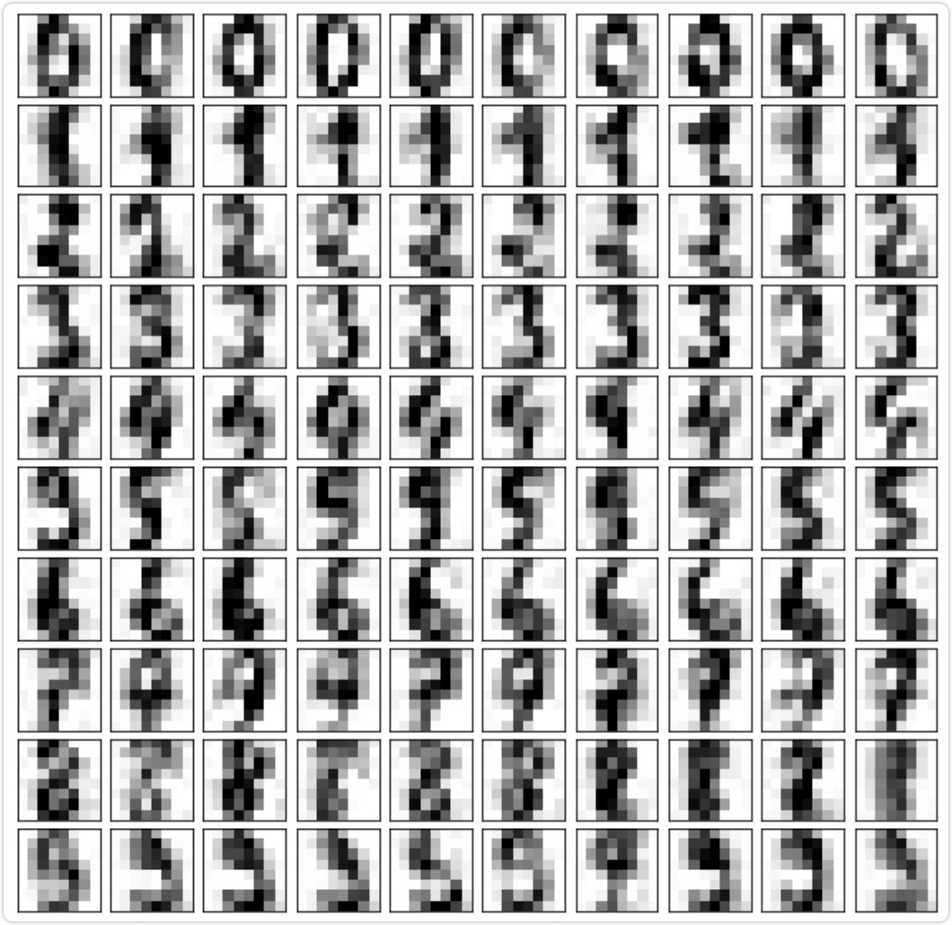
下面使用PCA进行降噪:
# 使用PCA降噪pca = PCA(0.5).fit(noisy_digits)pca.n_components_# 输出:12,即原始数据保存了50%的信息,需要12维# 进行降维、还原过程components = pca.transform(example_digits)filtered_digits = pca.inverse_transform(components)plot_digits(filtered_digits)
2 应用之人脸识别
PCA将样本X从n维空间映射到k维空间,求出前k个主成分,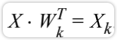 的矩阵,在经过主成分分析之后,一个k*n的主成分矩阵。如果将主成分矩阵也看成是由k个样本组成的矩阵,那么可以理解为第一个样本是最重要的样本,以此类推。
在人脸识别领域中,原始数据矩阵可以视为有m个人脸样本的集合,如果将主成分矩阵每一行也看做是一个样本的 话,每一行相当于是一个由原始人脸数据矩阵经过主成分分析得到的“特征脸”( Eigenface)矩阵,这个矩阵含有k 个“特征脸”。每个“特征脸”表达了原有样本中人脸的部分特征。
2.1 展示数据
# 2. 人脸识别import numpy as npimport matplotlib.pyplot as pltfrom sklearn.datasets import fetch_lfw_peoplefaces = fetch_lfw_people()print(faces.keys())# 输出:dict_keys('data', 'images','target','target_names','DESCR')print(faces.data.shape)# 输出:(13233,2914)# mages属性,即对每一维样本,将其以2维的形式展现出来# 即对于每个样本来说都是62*47print(faces.images.shape)# 输出:(13233,62,47)random_indexes = np.random.permutation(len(faces.data))X = faces.data[random_indexes]example_faces = X[:36, :]print(example_faces.shape)# 输出:(36,2914)# 一万多张脸抽出36张脸def plot_faces(faces):fig, axes = plt.subplots(6, 6, figsize=(10, 10),subplot_kw={'xticks': [], 'yticks': []},gridspec_kw=dict(hspace=0.1, wspace=0.1))for i, ax in enumerate(axes.flat):ax.imshow(faces[i].reshape(62, 47), cmap='bone')plt.show()plot_faces(example_faces)
在这里有一个小问题,就是数据集有可能下载不下来。
首先,看一下下载的目录,我的是mac电脑,这个包(fw funneled.tgz)被下载到了这个文件夹下面 /Users/your_name/scikit-learn data/tfw home/
把下载之前下载的文件fw funneled删除。(如果已经解压出文件夹,也把这个文件夹删除)
同时复制这个网址https://ndownloader.figshare.com/files/5976015到迅雷中,下载到完整的iwfunneded.tgz文件。并把这个文件复制到/ Users/ your name/ scikit_ Learn_data/ Lfw home/下面,并解压 缩。重新加载代码即可。
2.2 特征脸
# 特征脸from sklearn.decomposition import PCA%%time# 实例化PCA,求出所有的主成分pca = PCA(svd_solver='randomized')pca.fit(X)
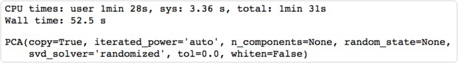
输出所有的主成分(向量)以及每个主成分的特征
print(pca.components_.shape)# 输出:(2914, 2914)
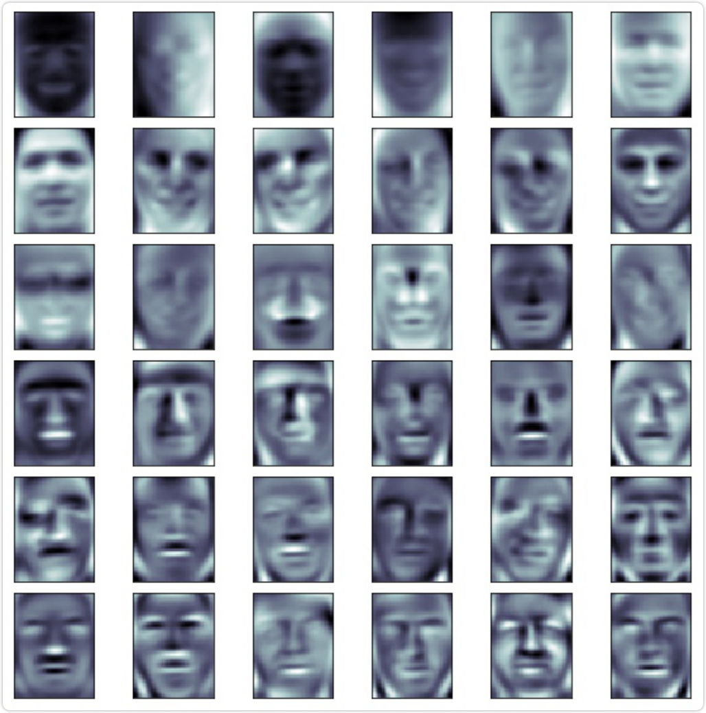
特征脸就是主成分中的每一行都当作一个样本,排名越靠前,表示该特征脸越能表示人脸的特征。取出前36个特征脸 进行可视化
plot_faces(pca.components_[:36, :])
3 总结
本篇文章介绍了主成分分析法的一些应用场景,除了降维以外,还可以进行降噪以及特征提取,也可以用作异常点检测
总之,PCA算法在机器学习领域中有非常广泛的应用,大家好好领悟其思想和原理,在应用中才会游刀有余

若有收获,就点个赞吧
0 人点赞
