开源算法包 - 异常点检测PyOD - 《机器学习-学习笔记》

一、PyOD介绍
二、PyOD主要亮点
三、工具库相关重要信息汇总：
四、作者介绍：
五、API介绍与实例（API References & Examples）
六、代码：
- 6.1 效果图

项目地址：https://github.com/yzhao062/Pyod#ramaswamy2000efficient
参考资料：
知乎-用PyOD工具库进行「异常检测」
使用PyOD库在Python中进行离群值检测
 PyOD在线文档
 CSDN-离群点异常检测及可视化分析工具pyod测试

一、PyOD介绍

异常检测（又称outlier detection、anomaly detection，离群值检测）是一种重要的数据挖掘方法，可以找到与“主要数据分布”不同的异常值（deviant from the general data distribution），比如从信用卡交易中找出诈骗案例，从正常的网络数据流中找出入侵，有非常广泛的商业应用价值。同时它可以被用于机器学习任务中的预处理（preprocessing），防止因为少量异常点存在而导致的训练或预测失败。

二、PyOD主要亮点

包括近20种常见的异常检测算法，比如经典的LOF/LOCI/ABOD以及最新的深度学习如对抗生成模型（GAN）和集成异常检测（outlier ensemble）
支持不同版本的Python：包括2.7和3.5+；支持多种操作系统：windows，macOS和Linux
简单易用且一致的API，只需要几行代码就可以完成异常检测，方便评估大量算法
使用JIT和并行化（parallelization）进行优化，加速算法运行及扩展性（scalability），可以处理大量数据

三、工具库相关重要信息汇总：

Github地址: pyod
PyPI下载地址: pyod
文档与API介绍（英文）: Welcome to PyOD documentation!
Jupyter Notebook示例（notebooks文件夹）: Binder (beta)
JMLR论文: PyOD: A Python Toolbox for Scalable Outlier Detection

四、作者介绍：

微调
数据挖掘 | 机器学习系统 | 前咨询师 | 在读博士
职业经历：
异常点检测PyOD - 图2 斯坦福大学 (Stanford University) · Visiting Student Researcher
异常点检测PyOD - 图3 艾昆纬 (IQVIA) · machine learning research intern
异常点检测PyOD - 图4 普华永道 · 高级数据科学家
教育经历：
异常点检测PyOD - 图5 卡内基梅隆大学 (Carnegie Mellon University) · 信息系统
异常点检测PyOD - 图6 多伦多大学 (University of Toronto) · 计算机科学
异常点检测PyOD - 图7 辛辛那提大学 · 计算机工程（CE）
异常点检测PyOD - 图8 山西省实验中学
个人简介
1. 机器学习系统架构师，参与设计了10个工具库/系统，GitHub Star>10000，下载量>300,0000
2. 生物制药 x 机器学习: https://github.com/mims-harvard/TDC
3. 大规模异常检测模型 SUOD：https://github.com/yzhao062/suod
4. PyOD异常检测工具库：https://github.com/yzhao062/pyod
5. 个人主页：https://www.andrew.cmu.edu/user/yuezhao2
6. GayHub: https://github.com/yzhao062
7. Google Scholar: https://scholar.google.com/cita

五、API介绍与实例（API References & Examples）

Examples可下载github项目中查看和运行。

特别需要注意的是，异常检测算法基本都是无监督学习，所以只需要X（输入数据），而不需要y（标签）。PyOD的使用方法和Sklearn中聚类分析很像，它的检测器（detector）均有统一的API。所有的PyOD检测器clf均有统一的API以便使用，完整的API使用参考可以查阅（API CheatSheet - pyod 0.6.8 documentation）：

fit(X): 用数据X来“训练/拟合”检测器clf。即在初始化检测器clf后，用X来“训练”它。
fit_predict_score(X, y): 用数据X来训练检测器clf，并预测X的预测值，并在真实标签y上进行评估。此处的y只是用于评估，而非训练
decision_function(X): 在检测器clf被fit后，可以通过该函数来预测未知数据的异常程度，返回值为原始分数，并非0和1。返回分数越高，则该数据点的异常程度越高
predict(X): 在检测器clf被fit后，可以通过该函数来预测未知数据的异常标签，返回值为二分类标签（0为正常点，1为异常点）
predict_proba(X): 在检测器clf被fit后，预测未知数据的异常概率，返回该点是异常点概率

当检测器clf被初始化且fit(X)函数被执行后，clf就会生成两个重要的属性：

decision_scores: 数据X上的异常打分，分数越高，则该数据点的异常程度越高
labels_: 数据X上的异常标签，返回值为二分类标签（0为正常点，1为异常点）

不难看出，当我们初始化一个检测器clf后，可以直接用数据X来“训练”clf，之后我们便可以得到X的异常分值（clf.decisionscores）以及异常标签（clf.labels）。当clf被训练后（当fit函数被执行后），我们可以使用decision_function()和predict()函数来对未知数据进行训练。
在有了背景知识后，我们可以使用PyOD来实现一个简单的异常检测实例：

from pyod.models.knn import KNN   # imprt kNN分类器
# 训练一个kNN检测器
clf_name = 'kNN'
clf = KNN() # 初始化检测器clf
clf.fit(X_train) # 使用X_train训练检测器clf
# 返回训练数据X_train上的异常标签和异常分值
y_train_pred = clf.labels_  # 返回训练数据上的分类标签 (0: 正常值, 1: 异常值)
y_train_scores = clf.decision_scores_  # 返回训练数据上的异常值 (分值越大越异常)
# 用训练好的clf来预测未知数据中的异常值
y_test_pred = clf.predict(X_test)  # 返回未知数据上的分类标签 (0: 正常值, 1: 异常值)
y_test_scores = clf.decision_function(X_test)  #  返回未知数据上的异常值 (分值越大越异常)

不难看出，PyOD的API和scikit-learn非常相似，只需要几行就可以得到数据的异常值。当检测器得到输出后，我们可以用以下代码评估其表现，或者直接可视化分类结果（图2）。

# 评估预测结果
print("\nOn Test Data:")
evaluate_print(clf_name, y_test, y_test_scores)
# 可视化
visualize(clf_name, X_train, y_train, X_test, y_test, y_train_pred,
    y_test_pred, show_figure=True, save_figure=False)

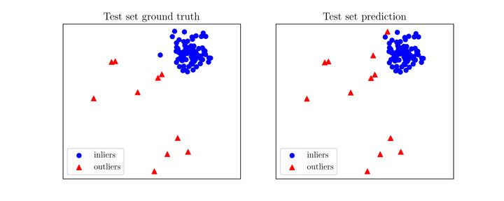异常点检测PyOD - 图10 图2. 预测结果（右图）与真实结果（左图）对比

六、代码：

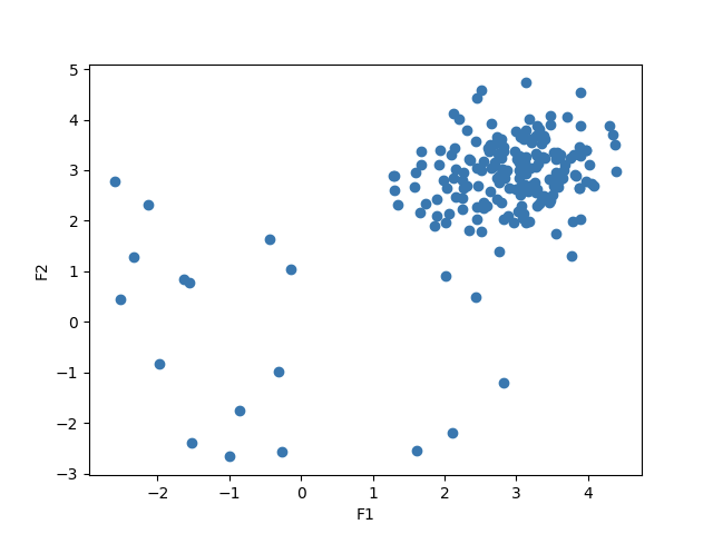
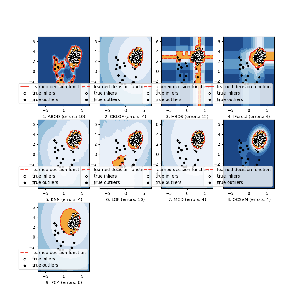
#!/usr/bin/env python
# -*- encoding: utf-8 -*-
"""
@File    :   outlierDetection.py    
@Modify Time      @Author    @Version    @Description
------------      -------    --------    -----------
2021/8/12 14:06   SeafyLiang   1.0       离群点检测pyod
"""
import numpy as np
from scipy import stats
import matplotlib.pyplot as plt
import matplotlib.font_manager
# 检测数据集中异常值的模型
from pyod.models.abod import ABOD
from pyod.models.cblof import CBLOF
# from pyod.models.feature_bagging import FeatureBagging
from pyod.models.hbos import HBOS
from pyod.models.iforest import IForest
from pyod.models.knn import KNN
# from pyod.models.loci import LOCI
# from pyod.models.sod import SOD
from pyod.models.lof import LOF
from pyod.models.mcd import MCD
from pyod.models.ocsvm import OCSVM
from pyod.models.pca import PCA
from pyod.utils.data import generate_data, get_outliers_inliers
"""
参考资料：
https://blog.csdn.net/weixin_41697507/article/details/89408236
https://blog.csdn.net/sparkexpert/article/details/81195418
https://github.com/yzhao062/Pyod#ramaswamy2000efficient
"""
# 创建一个带有异常值的随机数据集并绘制它
# generate random data with two features
X_train, Y_train = generate_data(n_train=200, train_only=True, n_features=2)
# by default the outlier fraction is 0.1 in generate data function
outlier_fraction = 0.1
# store outliers and inliers in different numpy arrays
x_outliers, x_inliers = get_outliers_inliers(X_train, Y_train)
n_inliers = len(x_inliers)
n_outliers = len(x_outliers)
# separate the two features and use it to plot the data
F1 = X_train[:, [0]].reshape(-1, 1)
F2 = X_train[:, [1]].reshape(-1, 1)
# create a meshgrid
xx, yy = np.meshgrid(np.linspace(-10, 10, 200), np.linspace(-10, 10, 200))
# scatter plot
plt.scatter(F1, F2)
plt.xlabel('F1')
plt.ylabel('F2')
plt.show()
"""
Model 1 Angle-based Outlier Detector (ABOD)
Model 2 Cluster-based Local Outlier Factor (CBLOF)
Model 3 Feature Bagging
Model 4 Histogram-base Outlier Detection (HBOS)
Model 5 Isolation Forest
Model 6 K Nearest Neighbors (KNN)
Model 7 Fast outlier detection using the local correlation integral(LOCI)
Model 8 Subspace Outlier Detection (SOD)
Model 9 Local Outlier Factor (LOF)
Model 10 Minimum Covariance Determinant (MCD)
Model 11 One-class SVM (OCSVM)
Model 12 Principal Component Analysis (PCA)
"""
# 创建一个dictionary并添加要用于检测异常值的所有模型
classifiers = {
    'ABOD': ABOD(contamination=outlier_fraction),
    'CBLOF': CBLOF(contamination=outlier_fraction),
    # 'Feature Bagging': FeatureBagging(contamination=outlier_fraction),
    'HBOS': HBOS(contamination=outlier_fraction),
    'IForest': IForest(contamination=outlier_fraction),
    'KNN': KNN(contamination=outlier_fraction),
    # 'LOCI': LOCI(contamination=outlier_fraction, ),
    # 'SOD': SOD(contamination=outlier_fraction, ),
    'LOF': LOF(contamination=outlier_fraction, ),
    'MCD': MCD(contamination=outlier_fraction, ),
    'OCSVM': OCSVM(contamination=outlier_fraction, ),
    'PCA': PCA(contamination=outlier_fraction, ),
}
# 将数据拟合到我们在dictionary中添加的每个模型，然后，查看每个模型如何检测异常值
# set the figure size
plt.figure(figsize=(10, 10))
for i, (clf_name, clf) in enumerate(classifiers.items()):
    print()
    print(i + 1, 'fitting', clf_name)
    # fit the data and tag outliers
    clf.fit(X_train)
    scores_pred = clf.decision_function(X_train) * -1
    y_pred = clf.predict(X_train)
    threshold = stats.scoreatpercentile(scores_pred,
                                        100 * outlier_fraction)
    n_errors = (y_pred != Y_train).sum()
    # plot the levels lines and the points
    Z = clf.decision_function(np.c_[xx.ravel(), yy.ravel()]) * -1
    Z = Z.reshape(xx.shape)
    subplot = plt.subplot(3, 4, i + 1)
    subplot.contourf(xx, yy, Z, levels=np.linspace(Z.min(), threshold, 7),
                     cmap=plt.cm.Blues_r)
    a = subplot.contour(xx, yy, Z, levels=[threshold],
                        linewidths=2, colors='red')
    subplot.contourf(xx, yy, Z, levels=[threshold, Z.max()],
                     colors='orange')
    b = subplot.scatter(X_train[:-n_outliers, 0], X_train[:-n_outliers, 1], c='white',
                        s=20, edgecolor='k')
    c = subplot.scatter(X_train[-n_outliers:, 0], X_train[-n_outliers:, 1], c='black',
                        s=20, edgecolor='k')
    subplot.axis('tight')
    subplot.legend(
        [a.collections[0], b, c],
        ['learned decision function', 'true inliers', 'true outliers'],
        prop=matplotlib.font_manager.FontProperties(size=10),
        loc='lower right')
    subplot.set_xlabel("%d. %s (errors: %d)" % (i + 1, clf_name, n_errors))
    subplot.set_xlim((-7, 7))
    subplot.set_ylim((-7, 7))
plt.show()

异常点检测PyOD