作者:Zuguang Gu8
翻译:Steven Shen
原文:https://jokergoo.github.io/ComplexHeatmap-reference/book/oncoprint.html#complex-alteration-types
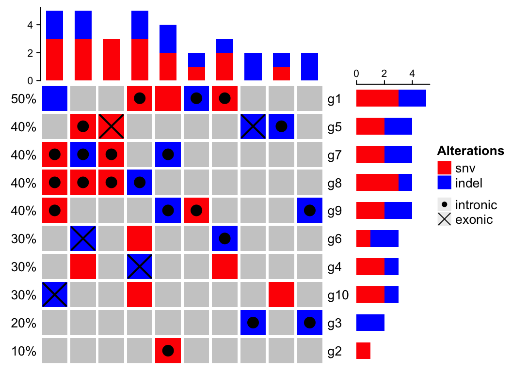
It is very easy to have many more different alteration types when integrating information from multiple analysis results. It is sometimes difficult to design graphics and assign different colors for them (e.g. see plot in this link. On the other hand, in these alteration types, there are primary classes of alteration types which is more important to distinguish, while there are secondary classes which is less important. For example, we may have alteration types of “intronic snv”, “exonic snv”, “intronic indel” and “exonic indel”. Actually we can classify them into two classes where “snv/indel” is more important and they belong to the primary class, and “intronic/exonic” is less important and they belong to the secondary class. Reflecting on the oncoPrint, for the “intronic snv” and “exonic snv”, we want to use similar graphics because they are snvs and we want them visually similar, and we add slightly different symbols to represent “intronic” and “exonic”, E.g. we can use red rectangle for snv and above the red rectangles, we use dots to represent “intronic” and cross lines to represent “exonic”. On the barplot annotations which summarize the number of different alteration types, we don’t want to separate “intronic snv” and “exonic snv” while we prefer to simply get the total number of snv to get rid of too many categories in the barplots.
Let’s demonstrate this scenario by following simulated data. To simplify the example, we assume for a single gene in a single sample, it only has either snv or indel and it can only be either intronic or exonic. If there is no “intronic” or “exonic” attached to the gene, it basically means we don’t have this gene-related information (maybe it is an intergenic snv/indel).
set.seed(123)x1 = sample(c("", "snv"), 100, replace = TRUE, prob = c(8, 2))x2 = sample(c("", "indel"), 100, replace = TRUE, prob = c(8, 2))x2[x1 == "snv"] = ""x3 = sample(c("", "intronic"), 100, replace = TRUE, prob = c(5, 5))x4 = sample(c("", "exonic"), 100, replace = TRUE, prob = c(5, 5))x3[x1 == "" & x2 == ""] = ""x4[x1 == "" & x2 == ""] = ""x4[x3 == "intronic"] = ""x = apply(cbind(x1, x2, x3, x4), 1, function(x) {x = x[x != ""]paste(x, collapse = ";")})m = matrix(x, nrow = 10, ncol = 10, dimnames = list(paste0("g", 1:10), paste0("s", 1:10)))m[1:4, 1:4]## s1 s2 s3 s4## g1 "" "snv;intronic" "snv;intronic" "snv"## g2 "" "" "" "snv;intronic"## g3 "" "" "" ""## g4 "snv" "indel;exonic" "snv" ""
Now in
m, there are four different alteration types:snv,indel,intronicandexonic. Next we definealter_funfor the four alterations.
alter_fun = list(background = function(x, y, w, h)grid.rect(x, y, w*0.9, h*0.9, gp = gpar(fill = "#CCCCCC", col = NA)),# red rectanglessnv = function(x, y, w, h)grid.rect(x, y, w*0.9, h*0.9, gp = gpar(fill = "red", col = NA)),# blue rectanglesindel = function(x, y, w, h)grid.rect(x, y, w*0.9, h*0.9, gp = gpar(fill = "blue", col = NA)),# dotsintronic = function(x, y, w, h)grid.points(x, y, pch = 16),# crossed linesexonic = function(x, y, w, h) {grid.segments(x - w*0.4, y - h*0.4, x + w*0.4, y + h*0.4, gp = gpar(lwd = 2))grid.segments(x + w*0.4, y - h*0.4, x - w*0.4, y + h*0.4, gp = gpar(lwd = 2))})
For the alteration types in the primary class (
snvandindel), we use colorred rectangles to represent them because the rectangles are visually obvious, while for the alteration types in the secondary class (intronicandexonic), we only use simple symbols (dots forintronicand crossed diagonal lines forexonic). Since there is no color corresponding tointronicandexonic, we don’t need to define colors for these two types, and on the barplot annotation for genes and samples, onlysnvandindelare visualized (so the height forsnvin the barplot corresponds the number of intronic snv plus exonic snv).In following code which draws the oncoPrint, we add another legend for the
intronic/exonictypes. note apchvalue of 16 corresponds to a dot and a value of 28 corresponds to crossed diagonal lines (see the last plot in Section 5.2 forpch26, 27, 28).
# we only define color for snv and indel, so barplot annotations only show snv and indelht = oncoPrint(m, alter_fun = alter_fun, col = c(snv = "red", indel = "blue"))draw(ht, heatmap_legend_list = list(Legend(labels = c("intronic", "exonic"), type = "points", pch = c(16, 28))))


