下面的范例使用Pytorch的低阶API实现线性回归模型和DNN二分类模型。
低阶API主要包括张量操作,计算图和自动微分。
import osimport datetime#打印时间def printbar():nowtime = datetime.datetime.now().strftime('%Y-%m-%d %H:%M:%S')print("\n"+"=========="*8 + "%s"%nowtime)#mac系统上pytorch和matplotlib在jupyter中同时跑需要更改环境变量os.environ["KMP_DUPLICATE_LIB_OK"]="TRUE"
线性回归模型
准备数据
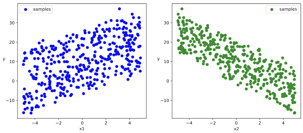
import numpy as npimport pandas as pdfrom matplotlib import pyplot as pltimport torchfrom torch import nn#样本数量n = 400# 生成测试用数据集X = 10*torch.rand([n,2])-5.0 #torch.rand是均匀分布w0 = torch.tensor([[2.0],[-3.0]])b0 = torch.tensor([[10.0]])Y = X@w0 + b0 + torch.normal( 0.0,2.0,size = [n,1]) # @表示矩阵乘法,增加正态扰动
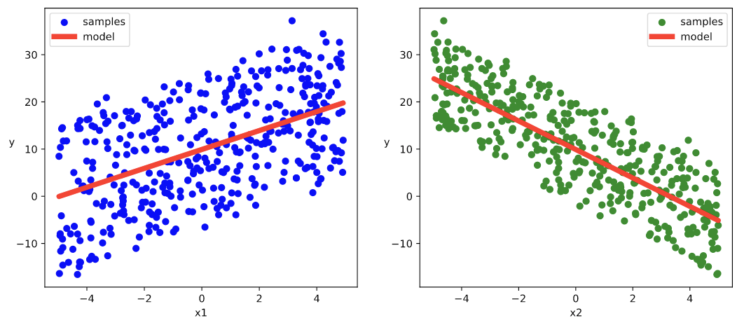
# 数据可视化%matplotlib inline%config InlineBackend.figure_format = 'svg'plt.figure(figsize = (12,5))ax1 = plt.subplot(121)ax1.scatter(X[:,0].numpy(),Y[:,0].numpy(), c = "b",label = "samples")ax1.legend()plt.xlabel("x1")plt.ylabel("y",rotation = 0)ax2 = plt.subplot(122)ax2.scatter(X[:,1].numpy(),Y[:,0].numpy(), c = "g",label = "samples")ax2.legend()plt.xlabel("x2")plt.ylabel("y",rotation = 0)plt.show()
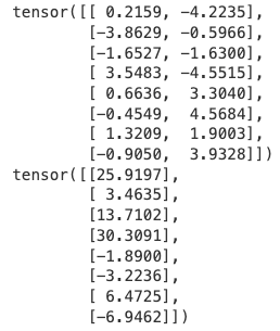
# 构建数据管道迭代器def data_iter(features, labels, batch_size=8):num_examples = len(features)indices = list(range(num_examples))np.random.shuffle(indices) #样本的读取顺序是随机的for i in range(0, num_examples, batch_size):indexs = torch.LongTensor(indices[i: min(i + batch_size, num_examples)])yield features.index_select(0, indexs), labels.index_select(0, indexs)# 测试数据管道效果batch_size = 8(features,labels) = next(data_iter(X,Y,batch_size))print(features)print(labels)
定义模型
# 定义模型class LinearRegression:def __init__(self):self.w = torch.randn_like(w0,requires_grad=True)self.b = torch.zeros_like(b0,requires_grad=True)#正向传播def forward(self,x):return x@self.w + self.b# 损失函数def loss_func(self,y_pred,y_true):return torch.mean((y_pred - y_true)**2/2)model = LinearRegression()
训练模型
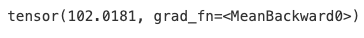
def train_step(model, features, labels):predictions = model.forward(features)loss = model.loss_func(predictions,labels)# 反向传播求梯度loss.backward()# 使用torch.no_grad()避免梯度记录,也可以通过操作 model.w.data 实现避免梯度记录with torch.no_grad():# 梯度下降法更新参数model.w -= 0.001*model.w.gradmodel.b -= 0.001*model.b.grad# 梯度清零model.w.grad.zero_()model.b.grad.zero_()return loss
# 测试train_step效果batch_size = 10(features,labels) = next(data_iter(X,Y,batch_size))train_step(model,features,labels)
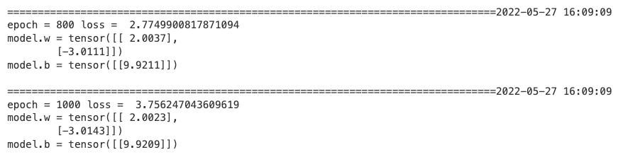
def train_model(model,epochs):for epoch in range(1,epochs+1):for features, labels in data_iter(X,Y,10):loss = train_step(model,features,labels)if epoch%200==0:printbar()print("epoch =",epoch,"loss = ",loss.item())print("model.w =",model.w.data)print("model.b =",model.b.data)train_model(model,epochs = 1000)
# 结果可视化%matplotlib inline%config InlineBackend.figure_format = 'svg'plt.figure(figsize = (12,5))ax1 = plt.subplot(121)ax1.scatter(X[:,0].numpy(),Y[:,0].numpy(), c = "b",label = "samples")ax1.plot(X[:,0].numpy(),(model.w[0].data*X[:,0]+model.b[0].data).numpy(),"-r",linewidth = 5.0,label = "model")ax1.legend()plt.xlabel("x1")plt.ylabel("y",rotation = 0)ax2 = plt.subplot(122)ax2.scatter(X[:,1].numpy(),Y[:,0].numpy(), c = "g",label = "samples")ax2.plot(X[:,1].numpy(),(model.w[1].data*X[:,1]+model.b[0].data).numpy(),"-r",linewidth = 5.0,label = "model")ax2.legend()plt.xlabel("x2")plt.ylabel("y",rotation = 0)plt.show()
DNN二分类模型
准备数据
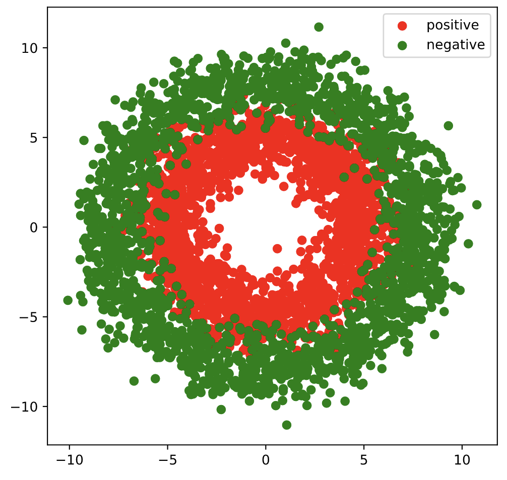
import numpy as npimport pandas as pdfrom matplotlib import pyplot as pltimport torchfrom torch import nn%matplotlib inline%config InlineBackend.figure_format = 'svg'#正负样本数量n_positive,n_negative = 2000,2000#生成正样本, 小圆环分布r_p = 5.0 + torch.normal(0.0,1.0,size = [n_positive,1])theta_p = 2*np.pi*torch.rand([n_positive,1])Xp = torch.cat([r_p*torch.cos(theta_p),r_p*torch.sin(theta_p)],axis = 1)Yp = torch.ones_like(r_p)#生成负样本, 大圆环分布r_n = 8.0 + torch.normal(0.0,1.0,size = [n_negative,1])theta_n = 2*np.pi*torch.rand([n_negative,1])Xn = torch.cat([r_n*torch.cos(theta_n),r_n*torch.sin(theta_n)],axis = 1)Yn = torch.zeros_like(r_n)#汇总样本X = torch.cat([Xp,Xn],axis = 0)Y = torch.cat([Yp,Yn],axis = 0)#可视化plt.figure(figsize = (6,6))plt.scatter(Xp[:,0].numpy(),Xp[:,1].numpy(),c = "r")plt.scatter(Xn[:,0].numpy(),Xn[:,1].numpy(),c = "g")plt.legend(["positive","negative"]);
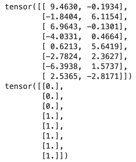
# 构建数据管道迭代器def data_iter(features, labels, batch_size=8):num_examples = len(features)indices = list(range(num_examples))np.random.shuffle(indices) #样本的读取顺序是随机的for i in range(0, num_examples, batch_size):indexs = torch.LongTensor(indices[i: min(i + batch_size, num_examples)])yield features.index_select(0, indexs), labels.index_select(0, indexs)# 测试数据管道效果batch_size = 8(features,labels) = next(data_iter(X,Y,batch_size))print(features)print(labels)
定义模型
此处范例我们利用nn.Module来组织模型变量。
class DNNModel(nn.Module):def __init__(self):super(DNNModel, self).__init__()self.w1 = nn.Parameter(torch.randn(2,4))self.b1 = nn.Parameter(torch.zeros(1,4))self.w2 = nn.Parameter(torch.randn(4,8))self.b2 = nn.Parameter(torch.zeros(1,8))self.w3 = nn.Parameter(torch.randn(8,1))self.b3 = nn.Parameter(torch.zeros(1,1))# 正向传播def forward(self,x):x = torch.relu(x@self.w1 + self.b1)x = torch.relu(x@self.w2 + self.b2)y = torch.sigmoid(x@self.w3 + self.b3)return y# 损失函数(二元交叉熵)def loss_func(self,y_pred,y_true):#将预测值限制在1e-7以上, 1- (1e-7)以下,避免log(0)错误eps = 1e-7y_pred = torch.clamp(y_pred,eps,1.0-eps)bce = - y_true*torch.log(y_pred) - (1-y_true)*torch.log(1-y_pred)return torch.mean(bce)# 评估指标(准确率)def metric_func(self,y_pred,y_true):y_pred = torch.where(y_pred>0.5,torch.ones_like(y_pred,dtype = torch.float32),torch.zeros_like(y_pred,dtype = torch.float32))acc = torch.mean(1-torch.abs(y_true-y_pred))return accmodel = DNNModel()
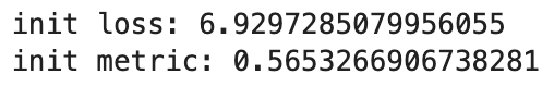
# 测试模型结构batch_size = 10(features,labels) = next(data_iter(X,Y,batch_size))predictions = model(features)loss = model.loss_func(labels,predictions)metric = model.metric_func(labels,predictions)print("init loss:", loss.item())print("init metric:", metric.item())
len(list(model.parameters()))

训练模型
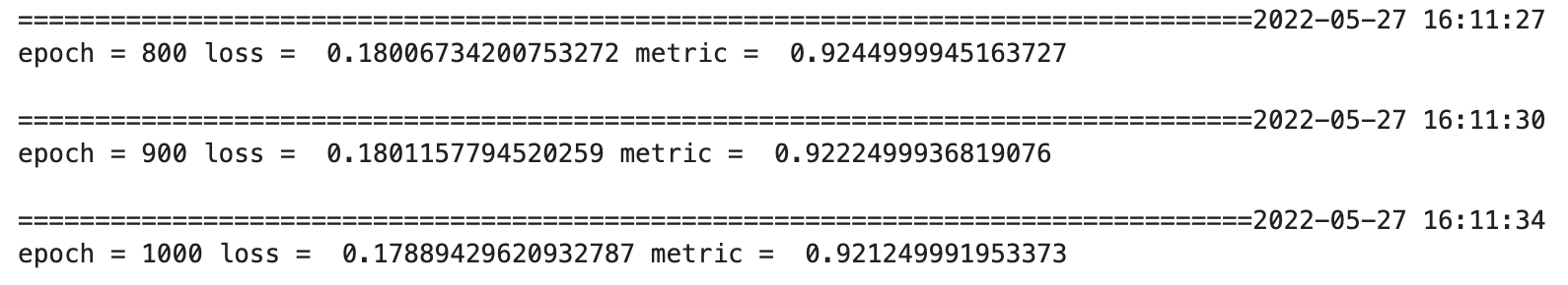
def train_step(model, features, labels):# 正向传播求损失predictions = model.forward(features)loss = model.loss_func(predictions,labels)metric = model.metric_func(predictions,labels)# 反向传播求梯度loss.backward()# 梯度下降法更新参数for param in model.parameters():#注意是对param.data进行重新赋值,避免此处操作引起梯度记录param.data = (param.data - 0.01*param.grad.data)# 梯度清零model.zero_grad()return loss.item(),metric.item()def train_model(model,epochs):for epoch in range(1,epochs+1):loss_list,metric_list = [],[]for features, labels in data_iter(X,Y,20):lossi,metrici = train_step(model,features,labels)loss_list.append(lossi)metric_list.append(metrici)loss = np.mean(loss_list)metric = np.mean(metric_list)if epoch%100==0:printbar()print("epoch =",epoch,"loss = ",loss,"metric = ",metric)train_model(model,epochs = 1000)
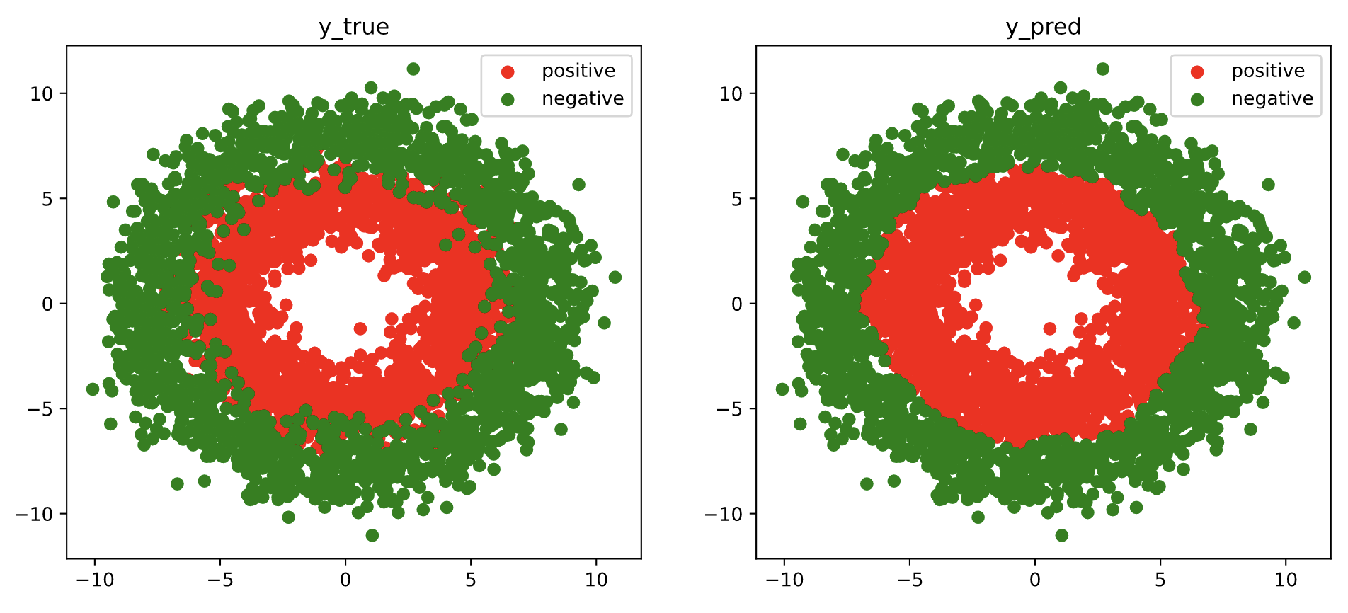
# 结果可视化fig, (ax1,ax2) = plt.subplots(nrows=1,ncols=2,figsize = (12,5))ax1.scatter(Xp[:,0],Xp[:,1], c="r")ax1.scatter(Xn[:,0],Xn[:,1],c = "g")ax1.legend(["positive","negative"]);ax1.set_title("y_true");Xp_pred = X[torch.squeeze(model.forward(X)>=0.5)]Xn_pred = X[torch.squeeze(model.forward(X)<0.5)]ax2.scatter(Xp_pred[:,0],Xp_pred[:,1],c = "r")ax2.scatter(Xn_pred[:,0],Xn_pred[:,1],c = "g")ax2.legend(["positive","negative"]);ax2.set_title("y_pred");

若有收获,就点个赞吧
0 人点赞
