[MobileNet]MobileNet理解

参考见图片水印。很早之前的一个笔记，当时看了比较多的博客整理的，最近重温轻量化网络结构设计就把笔记迁到语雀上。

一、理论梳理

轻量化网络：MobileNet-V2

1.1 mobileNet v1

参考文献：

• 轻量级网络—MobileNet论文解读

最主要的贡献在于深度可分离卷积和点卷积（即1*1的卷积）

深度可分离卷积干的活是：把标准卷积分解成深度卷积(depthwise convolution)和逐点卷积(pointwise convolution)。这么做的好处是可以大幅度降低参数量和计算量。
分解过程示意图如下：

图1.1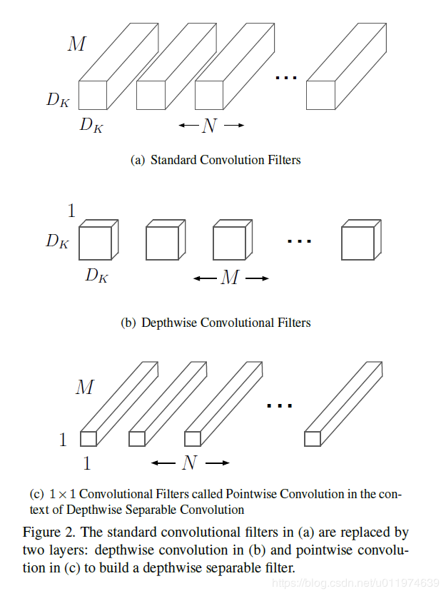

对这个图进行一波分析。输入是D_F*D_F*M时，M表示通道数。
传统卷积的卷积核会设为D_K*D_K*M，一共有N个这样的卷积核，得到最终输出是D_F*D_F*N。计算时也是直接逐个通道对应元素累乘再累加，再将每个通道对应位置进行累加（有时还需加上偏置项）。如图1.2所示。

图1.2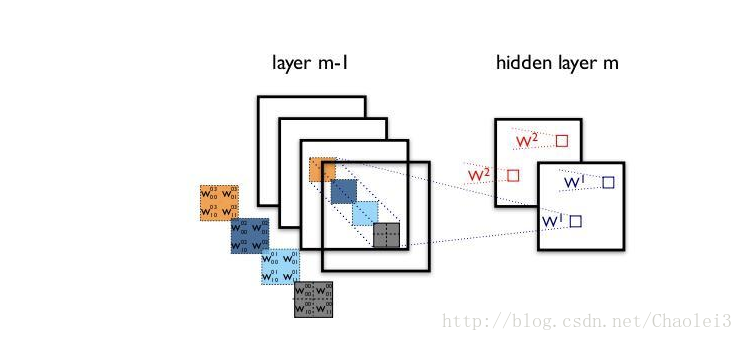

而深度可分离卷积是这样的，它分成了两个卷积步骤，首先深度卷积，卷积核设置为D_K*D_K*1，一共有M个这样的卷积核，即每个通道对应一个卷积核，此时得到的输出是D_F*D_F*M。再用点卷积，即1*1*M的卷积核，共N个，得到最终输出D_F*D_F*N。如图1.3所示。

图1.3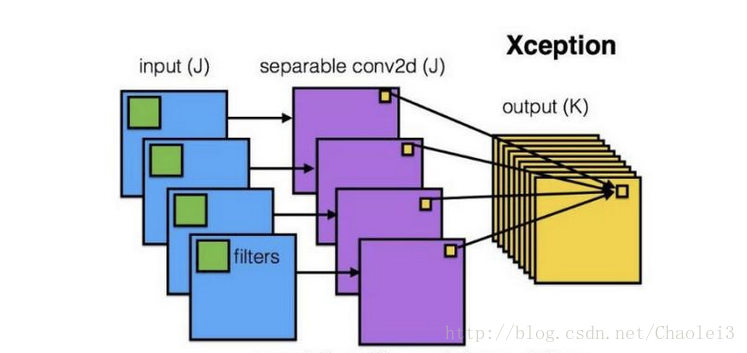

再放些好图

图1.4

这里就是a和b的区别了。3和4是v2的改进点

下面来一波计算。
假设：

1. 输入特征图大小为 D_F*D_F*M
2. 输出特征图大小为 D_F*D_F*N
3. 卷积核大小为 D_K*D_K

那么我们可以计算得到

1. 传统卷积的计算量为：D_F * D_F * N * D_K * D_K * N
   (道理是：一共有D_F * D_F * N个结果，每个结果需要经过D_K * D_K * N次计算）
   参数量：D_F*D_F*N
2. 深度可分离卷积第一次卷积的计算量是D_F * D_F * M * D_K * D_K，
   第二次卷积的计算量是D_F * D_F * N * M，
   总计算量是D_F * D_F * M * D_K * D_K + D_F * D_F * N * M。
   参数量：D_K*D_K*1*M + 1*1*M*N

两种卷积方法的计算量差别是：

参数量的差别是：

以作者论文中 28×28×192 的输入，28×28×256 的输出为例，卷积核大小为 3×3，两者的计算量之比为：

深度可分离卷积的计算量缩减为传统卷积的 1/9 左右。

1.2 mobileNet v2

参考文献

• 轻量化网络：MobileNet-V2这个超棒
• 轻量级网络—MobileNetV2论文解读有点晦涩

v2的创新点：

1. Inverted residuals，通常的residuals block是先经过一个1*1的Conv layer，把feature map的通道数“压”下来，再经过3*3Conv layer，最后经过一个1*1的Conv layer，将feature map通道数再“扩张”回去。即先“压缩”，最后“扩张”回去。
   （而 inverted residuals就是 先“扩张”，最后“压缩”。为什么这么做呢？请往下看。）
2. Linear bottlenecks，为了避免Relu对特征的破坏，在residual block的Eltwise sum之前的那个 1*1 Conv 不再采用Relu。（为什么？请往下看。）

用一图说明这两个创新。

图1.5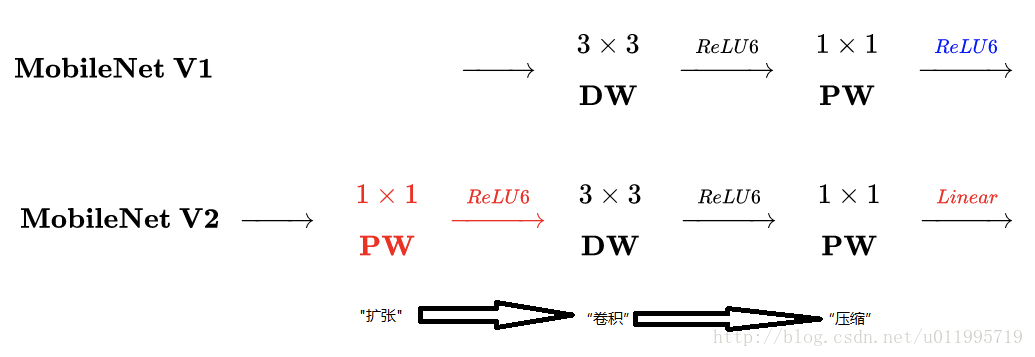

MobileNet-V1 最大的特点就是采用depth-wise separable convolution来减少运算量以及参数量，而在网络结构上，没有采用shortcut的方式。
当时Resnet及Densenet等一系列采用shortcut的网络的成功，表明了shortcut是个非常好的东西，于是MobileNet-V2就将这个好东西拿来用。

MobileNet的特点就是depth-wise separable convolution，但是直接把depth-wise separable convolution应用到 residual block中，会碰到如下问题：

1. DWConv layer层提取得到的特征受限于输入的通道数，若是采用以往的residual block，先“压缩”，再卷积提特征，那么DWConv layer可提取得特征就太少了，因此一开始不“压缩”，MobileNetV2反其道而行，一开始先“扩张”，本文实验“扩张”倍数为6。 通常residual block里面是 “压缩”→“卷积提特征”→“扩张”，MobileNetV2就变成了 “扩张”→“卷积提特征”→ “压缩”，因此称为Inverted residuals
2. 当采用“扩张”→“卷积提特征”→ “压缩”时，在“压缩”之后会碰到一个问题，那就是Relu会破坏特征。为什么这里的Relu会破坏特征呢？这得从Relu的性质说起，Relu对于负的输入，输出全为零；而本来特征就已经被“压缩”，再经过Relu的话，又要“损失”一部分特征，因此这里不采用Relu，实验结果表明这样做是正确的，这就称为Linear bottlenecks

这时候需要重新把一张图翻出来讲了。
图1.4

• 图(a)：普通模型架构使用标准卷积将空间和通道信息一起映射到下一层，参数和计算量会比较大
• 图(b)，MobileNetv1中将标准卷积拆分为深度卷积和逐点卷积，深度卷积负责逐通道的过滤空间信息，逐点卷积负责映射通道。将空间和通道分开了
• 图(c)和图(d)是MobileNetv2的结构(d是c的下一个连接状态)，同样是将标准卷积拆分为深度卷积和逐点卷积，在逐点卷积后使用了接1×1卷积，该卷积使用线性变换，总称为一层低维linear bottleneck，其作用是将输入映射回低维空间

映射完成以后使用shortcut，即残差网络
图1.5.1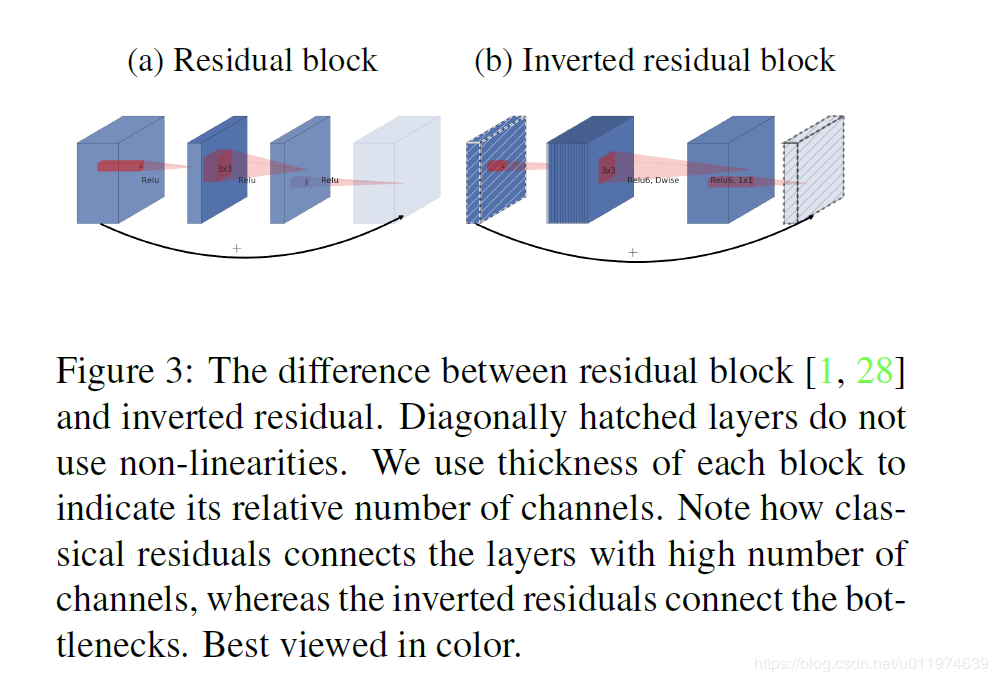

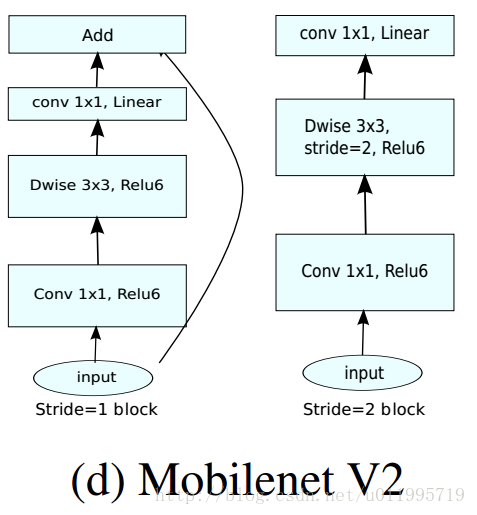
一个正经的bottleneck由下图构成

图1.6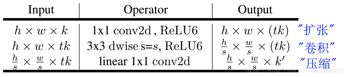

• 首先是1×1 conv2d变换通道，后接ReLU6激活(ReLU6即最高输出为6，超过了会clip下来)
• 中间是深度卷积,后接ReLU
• 最后的1×1 conv2d后面不接ReLU了，而是论文提出的linear bottleneck

针对stride=1和2，有不同的处理方法。为了与shortcut的维度匹配，stride=2时，不采用shortcut。

图1.7

二、代码梳理

2.1 深度可分离卷积

用pytorch实现比较简单，conv2d中有个参数叫groups，将它设置为通道数即可

2.2 源码

Randl/MobileNetV2-pytorch我的shuffleNet就是看他的代码
tonylins/pytorch-mobilenet-v2

看几个关键block

InvertedResidual

图2.1 网络结构图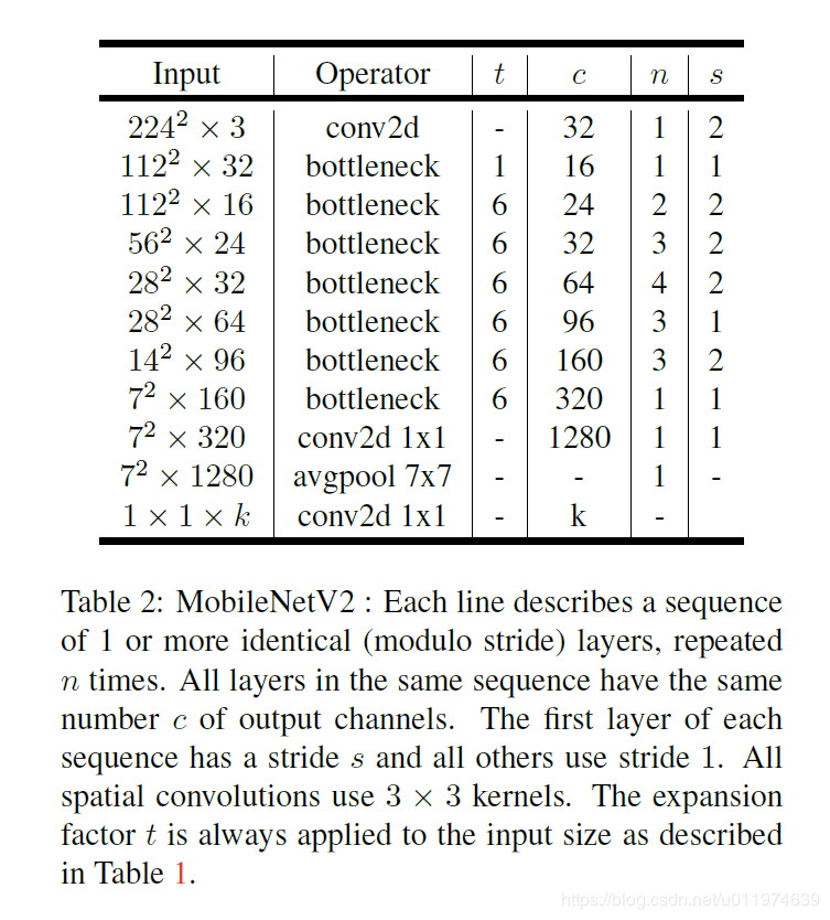

其中：t表示“扩张”倍数，c表示输出通道数，n表示重复次数，s表示步长stride。
先说两点有误之处吧：

1. 第五行，也就是第7~10个bottleneck，stride=2，分辨率应该从28降低到14；如果不是分辨率出错，那就应该是stride=1；
2. 文中提到共计采用19个bottleneck，但是这里只有17个。

class InvertedResidual(nn.Module):
    # inputSize, outputSize, stride和扩张倍数
    def __init__(self, inp, oup, stride, expand_ratio):
        super(InvertedResidual, self).__init__()
        self.stride = stride
        assert stride in [1, 2]
        hidden_dim = round(inp * expand_ratio)
        # 判断是否需要shortcut
        self.use_res_connect = self.stride == 1 and inp == oup
        # 如果不需要扩张, 则步骤为：3*3的DWconv->BN->Relu6->1*1的PWConv->BN
        if expand_ratio == 1:
            self.conv = nn.Sequential(
                # dw 深度可分离卷积
                # torch.nn.Conv2d(in_channels, out_channels, kernel_size, stride=1, padding=0, dilation=1, groups=1, bias=True)
                nn.Conv2d(hidden_dim, hidden_dim, 3, stride, 1, groups=hidden_dim, bias=False),
                nn.BatchNorm2d(hidden_dim),
                nn.ReLU6(inplace=True),
                # pw-linear 点卷积，实现线性变换
                # 点卷积不需要padding
                nn.Conv2d(hidden_dim, oup, 1, 1, 0, bias=False),
                nn.BatchNorm2d(oup),
            )
        # 如果需要扩张，则步骤为图1.7所示
        # 1*1 PWconv->BN->Relu6->3*3 DWconv->BN->Relu6->1*1 PWconv->BN
        else:
            self.conv = nn.Sequential(
                # pw
                nn.Conv2d(inp, hidden_dim, 1, 1, 0, bias=False),
                nn.BatchNorm2d(hidden_dim),
                nn.ReLU6(inplace=True),
                # dw
                nn.Conv2d(hidden_dim, hidden_dim, 3, stride, 1, groups=hidden_dim, bias=False),
                nn.BatchNorm2d(hidden_dim),
                nn.ReLU6(inplace=True),
                # pw-linear
                nn.Conv2d(hidden_dim, oup, 1, 1, 0, bias=False),
                nn.BatchNorm2d(oup),
            )
    def forward(self, x):
        if self.use_res_connect:
            return x + self.conv(x)
        else:
            return self.conv(x)

另一种写法。可以发现两者是有区别的。上面的方法单独考虑了扩张倍数是1，上文的做法是3*3的DWconv->BN->Relu6->1*1的PWConv->BN
而这里的做法没考虑，还是普遍做法，1*1 PWconv->BN->Relu6->3*3 DWconv->BN->Relu6->1*1 PWconv->BN
原因是因为在MobileNet的主函数里面，一个会单独建Module，另一个把它作为通用模块

class LinearBottleneck(nn.Module):
    # inputSize, outputSize, stride, t是扩张倍数，激活函数
    def __init__(self, inplanes, outplanes, stride=1, t=6, activation=nn.ReLU6):
        super(LinearBottleneck, self).__init__()
        self.conv1 = nn.Conv2d(inplanes, inplanes * t, kernel_size=1, bias=False)
        self.bn1 = nn.BatchNorm2d(inplanes * t)
        self.conv2 = nn.Conv2d(inplanes * t, inplanes * t, kernel_size=3, stride=stride, padding=1, bias=False,
                               groups=inplanes * t)
        self.bn2 = nn.BatchNorm2d(inplanes * t)
        self.conv3 = nn.Conv2d(inplanes * t, outplanes, kernel_size=1, bias=False)
        self.bn3 = nn.BatchNorm2d(outplanes)
        self.activation = activation(inplace=True)
        self.stride = stride
        self.t = t
        self.inplanes = inplanes
        self.outplanes = outplanes
    def forward(self, x):
        residual = x
        # 1*1 PWconv->BN->Relu6
        out = self.conv1(x)
        out = self.bn1(out)
        out = self.activation(out)
        # 3*3 DWconv->BN->Relu6
        out = self.conv2(out)
        out = self.bn2(out)
        out = self.activation(out)
        # 1*1 PWconv->BN
        out = self.conv3(out)
        out = self.bn3(out)
        # 根据stride决定是否需要残差
        if self.stride == 1 and self.inplanes == self.outplanes:
            out += residual
        return out

MobileNetV2

下文中出现了一个参数width_mult，这是什么呢～让我们重温这张图
图2.1 网络结构图

注意最下面一行的k了吗？MobileNetV1中提出了宽度缩放因子，其作用是在整体上对网络的每一层维度（特征数量）进行瘦身。MobileNetV2中，当该因子<1时，最后的那个1*1conv不进行宽度缩放；否则进行宽度缩放。

class MobileNetV2(nn.Module):
    # 输出类别，输入尺寸，宽度缩放因子
    def __init__(self, n_class=1000, input_size=224, width_mult=1.):
        super(MobileNetV2, self).__init__()
        block = InvertedResidual
        # 这两个数据是从论文中来的，如图2.1
        input_channel = 32
        last_channel = 1280
        # 根据作者的论文数据来的，如图2.1
        interverted_residual_setting = [
            # t, c, n, s
            [1, 16, 1, 1],
            [6, 24, 2, 2],
            [6, 32, 3, 2],
            [6, 64, 4, 2],
            [6, 96, 3, 1],
            [6, 160, 3, 2],
            [6, 320, 1, 1],
        ]
        # building first layer
        assert input_size % 32 == 0
        input_channel = int(input_channel * width_mult)
        self.last_channel = int(last_channel * width_mult) if width_mult > 1.0 else last_channel
        self.features = [conv_bn(3, input_channel, 2)]
        # building inverted residual blocks
        for t, c, n, s in interverted_residual_setting:
        # t表示“扩张”倍数，c表示输出通道数，n表示重复次数，s表示步长stride。
            output_channel = int(c * width_mult)
            # 这一部分的意思是先按s来一个，剩下的stride都是1
            for i in range(n):
                if i == 0:
                    self.features.append(block(input_channel, output_channel, s, expand_ratio=t))
                else:
                    self.features.append(block(input_channel, output_channel, 1, expand_ratio=t))
                input_channel = output_channel
        # building last several layers
        # 在多个bottleneck后有一个pw conv, 具体包括1*1conv->BN->relu6
        self.features.append(conv_1x1_bn(input_channel, self.last_channel))
        # make it nn.Sequential
        # 之前的self.features里面存的是list，现在要把它改成Sequential
        # 问题：为什么要有这个*不是很理解
        self.features = nn.Sequential(*self.features)
        # building classifier
        # 问题：整套流程下来好像少了一个Avgpool
        # 问题已解决，AvgPool用自己的方式实现在forward里了
        self.classifier = nn.Sequential(
            nn.Dropout(0.2),
            nn.Linear(self.last_channel, n_class),
        )
        self._initialize_weights()
    def forward(self, x):
        x = self.features(x)
        x = x.mean(3).mean(2)
        x = self.classifier(x)
        return x
    def _initialize_weights(self):
        for m in self.modules():
            if isinstance(m, nn.Conv2d):
                n = m.kernel_size[0] * m.kernel_size[1] * m.out_channels
                m.weight.data.normal_(0, math.sqrt(2. / n))
                if m.bias is not None:
                    m.bias.data.zero_()
            elif isinstance(m, nn.BatchNorm2d):
                m.weight.data.fill_(1)
                m.bias.data.zero_()
            elif isinstance(m, nn.Linear):
                n = m.weight.size(1)
                m.weight.data.normal_(0, 0.01)
                m.bias.data.zero_()

class MobileNet2(nn.Module):
    """MobileNet2 implementation.
    """
    # scale：缩放因子，t是扩张倍数
    def __init__(self, scale=1.0, input_size=224, t=6, in_channels=3, num_classes=1000, activation=nn.ReLU6):
        """
        MobileNet2 constructor.
        :param in_channels: (int, optional): number of channels in the input tensor.
                Default is 3 for RGB image inputs.
        :param input_size:
        :param num_classes: number of classes to predict. Default
                is 1000 for ImageNet.
        :param scale:
        :param t:
        :param activation:
        """
        super(MobileNet2, self).__init__()
        self.scale = scale
        self.t = t
        self.activation_type = activation
        self.activation = activation(inplace=True)
        self.num_classes = num_classes
        self.num_of_channels = [32, 16, 24, 32, 64, 96, 160, 320]
        # assert (input_size % 32 == 0)
        # 这里的_make_divisible和shuffleNet V2里的辅助函数一致，都是为了让输入能被分组数整除
        self.c = [_make_divisible(ch * self.scale, 8) for ch in self.num_of_channels]
        self.n = [1, 1, 2, 3, 4, 3, 3, 1]
        self.s = [2, 1, 2, 2, 2, 1, 2, 1]
        # 这里完成了bottleNeck之前的结构：conv->BN
        self.conv1 = nn.Conv2d(in_channels, self.c[0], kernel_size=3, bias=False, stride=self.s[0], padding=1)
        self.bn1 = nn.BatchNorm2d(self.c[0])
        # 这里完成了bottleNeck
        self.bottlenecks = self._make_bottlenecks()
        # Last convolution has 1280 output channels for scale <= 1
        self.last_conv_out_ch = 1280 if self.scale <= 1 else _make_divisible(1280 * self.scale, 8)
        self.conv_last = nn.Conv2d(self.c[-1], self.last_conv_out_ch, kernel_size=1, bias=False)
        self.bn_last = nn.BatchNorm2d(self.last_conv_out_ch)
        # AdaptiveAvgPool2d全局池化的作用
        self.avgpool = nn.AdaptiveAvgPool2d(1)
        self.dropout = nn.Dropout(p=0.2, inplace=True)  # confirmed by paper authors
        self.fc = nn.Linear(self.last_conv_out_ch, self.num_classes)
        self.init_params()
    def init_params(self):
        for m in self.modules():
            if isinstance(m, nn.Conv2d):
                init.kaiming_normal_(m.weight, mode='fan_out')
                if m.bias is not None:
                    init.constant_(m.bias, 0)
            elif isinstance(m, nn.BatchNorm2d):
                init.constant_(m.weight, 1)
                init.constant_(m.bias, 0)
            elif isinstance(m, nn.Linear):
                init.normal_(m.weight, std=0.001)
                if m.bias is not None:
                    init.constant_(m.bias, 0)
    def _make_stage(self, inplanes, outplanes, n, stride, t, stage):
        modules = OrderedDict()
        stage_name = "LinearBottleneck{}".format(stage)
        # First module is the only one utilizing stride
        first_module = LinearBottleneck(inplanes=inplanes, outplanes=outplanes, stride=stride, t=t,
                                        activation=self.activation_type)
        modules[stage_name + "_0"] = first_module
        # add more LinearBottleneck depending on number of repeats
        for i in range(n - 1):
            name = stage_name + "_{}".format(i + 1)
            module = LinearBottleneck(inplanes=outplanes, outplanes=outplanes, stride=1, t=6,
                                      activation=self.activation_type)
            modules[name] = module
        return nn.Sequential(modules)
    # 对于BottleNec，第一层BottleNec单独写了，之后的用了一个循环，扩张倍数默认是6
    def _make_bottlenecks(self):
        modules = OrderedDict()
        stage_name = "Bottlenecks"
        # First module is the only one with t=1
        bottleneck1 = self._make_stage(inplanes=self.c[0], outplanes=self.c[1], n=self.n[1], stride=self.s[1], t=1,
                                       stage=0)
        modules[stage_name + "_0"] = bottleneck1
        # add more LinearBottleneck depending on number of repeats
        for i in range(1, len(self.c) - 1):
            name = stage_name + "_{}".format(i)
            module = self._make_stage(inplanes=self.c[i], outplanes=self.c[i + 1], n=self.n[i + 1],
                                      stride=self.s[i + 1],
                                      t=self.t, stage=i)
            modules[name] = module
        return nn.Sequential(modules)
    def forward(self, x):
        x = self.conv1(x)
        x = self.bn1(x)
        x = self.activation(x)
        x = self.bottlenecks(x)
        x = self.conv_last(x)
        x = self.bn_last(x)
        x = self.activation(x)
        # average pooling layer
        x = self.avgpool(x)
        x = self.dropout(x)
        # flatten for input to fully-connected layer
        x = x.view(x.size(0), -1)
        x = self.fc(x)
        return F.log_softmax(x, dim=1) #TODO not needed(?)