原文:How to Build Exponential Smoothing Models Using Python: Simple Exponential Smoothing, Holt, and…
需要用到 statsmodels 这个包。
import matplotlib.pyplot as pltfrom statsmodels.tsa.holtwinters import ExponentialSmoothing, SimpleExpSmoothing, Holt
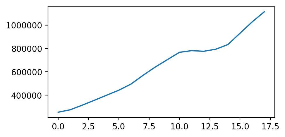
示例中的源数据:
data = [253993,275396.2,315229.5,356949.6,400158.2,442431.7,495102.9,570164.8,640993.1,704250.4,767455.4,781807.8,776332.3,794161.7,834177.7,931651.5,1028390,1114914]plt.plot(data);
简单指数平滑(SES)
对于没有明显趋势或季节规律的预测数据,SES 是一个很好的选择。预测是使用加权平均来计算的,这意味着最大的权重与最近的观测值相关,而最小的权重与最远的观测值相关

其中 0≤α≤1 是平滑参数。
权重减小率由平滑参数 α 控制。 如果 α 很大(即接近1),则对更近期的观察给予更多权重。 有两种极端情况:
- α= 0:所有未来值的预测等于历史数据的平均值(或“平均值”),称为平均值法。
- α= 1:简单地将所有预测设置为最后一次观测的值,统计中称为朴素方法。
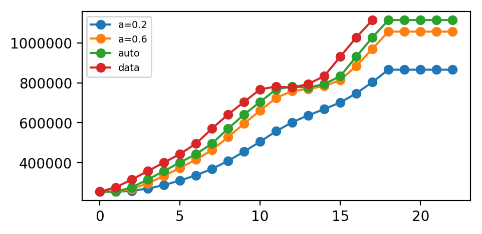
这里我们运行三种简单指数平滑变体:
- 在fit1中,我们明确地为模型提供了平滑参数α=0.2
- 在fit2中,我们选择α=0.6
- 在fit3中,我们使用自动优化,允许statsmodels自动为我们找到优化值。 这是推荐的方法。
# Simple Exponential Smoothingfit1 = SimpleExpSmoothing(data).fit(smoothing_level=0.2,optimized=False)# plotl1, = plt.plot(list(fit1.fittedvalues) + list(fit1.forecast(5)), marker='o')fit2 = SimpleExpSmoothing(data).fit(smoothing_level=0.6,optimized=False)# plotl2, = plt.plot(list(fit2.fittedvalues) + list(fit2.forecast(5)), marker='o')fit3 = SimpleExpSmoothing(data).fit()# plotl3, = plt.plot(list(fit3.fittedvalues) + list(fit3.forecast(5)), marker='o')l4, = plt.plot(data, marker='o')plt.legend(handles = [l1, l2, l3, l4], labels = ['a=0.2', 'a=0.6', 'auto', 'data'], loc = 'best', prop={'size': 7})plt.show()# 我们预测了未来五个点
Holt’s 方法(二次指数平滑)
Holt扩展了简单的指数平滑(数据解决方案没有明确的趋势或季节性),以便在1957年预测数据趋势。Holt的方法包括预测方程和两个平滑方程(一个用于水平,一个用于趋势):

其中0≤α≤1是水平平滑参数,0≤β∗≤1是趋势平滑参数。
对于长期预测,使用Holt方法的预测在未来会无限期地增加或减少。 在这种情况下,我们使用具有阻尼参数0<φ<1的阻尼趋势方法来防止预测“失控”。

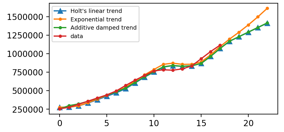
同样,这里我们运行Halt方法的三种变体:
- 在
fit1中,我们明确地为模型提供了平滑参数α=0.8,β∗=0.2。 - 在
fit2中,我们使用指数模型而不是Holt的加法模型(默认值)。 - 在
fit3中,我们使用阻尼版本的Holt附加模型,但允许优化阻尼参数φ,同时固定α=0.8,β∗=0.2的值。
data_sr = pd.Series(data)# Holt’s Methodfit1 = Holt(data_sr).fit(smoothing_level=0.8, smoothing_slope=0.2, optimized=False)l1, = plt.plot(list(fit1.fittedvalues) + list(fit1.forecast(5)), marker='^')fit2 = Holt(data_sr, exponential=True).fit(smoothing_level=0.8, smoothing_slope=0.2, optimized=False)l2, = plt.plot(list(fit2.fittedvalues) + list(fit2.forecast(5)), marker='.')fit3 = Holt(data_sr, damped=True).fit(smoothing_level=0.8, smoothing_slope=0.2)l3, = plt.plot(list(fit3.fittedvalues) + list(fit3.forecast(5)), marker='.')l4, = plt.plot(data_sr, marker='.')plt.legend(handles = [l1, l2, l3, l4], labels = ["Holt's linear trend", "Exponential trend", "Additive damped trend", 'data'], loc = 'best', prop={'size': 7})plt.show()
Holt-Winters 方法(三次指数平滑)
(彼得·温特斯(Peter Winters)是霍尔特(Holt)的学生。霍尔特-温特斯法最初是由彼得提出的,后来他们一起研究。
Holt-Winters的方法适用于具有趋势和季节性的数据,其包括季节性平滑参数γγ。 此方法有两种变体:
- 加法方法:整个序列的季节变化基本保持不变。
- 乘法方法:季节变化与系列水平成比例变化。
在这里,我们运行完整的Holt-Winters方法,包括趋势组件和季节性组件。 Statsmodels允许所有组合,包括如下面的示例所示:
- 在
fit1中,我们使用加法趋势,周期season_length = 4的加性季节和Box-Cox变换。 - 在
fit2中,我们使用加法趋势,周期season_length = 4的乘法季节和Box-Cox变换。 - 在
fit3中,我们使用加性阻尼趋势,周期season_length = 4的加性季节和Box-Cox变换。 - 在
fit4中,我们使用加性阻尼趋势,周期season_length = 4的乘法季节和Box-Cox变换。
data_sr = pd.Series(data)fit1 = ExponentialSmoothing(data_sr, seasonal_periods=4, trend='add', seasonal='add').fit(use_boxcox=True)fit2 = ExponentialSmoothing(data_sr, seasonal_periods=4, trend='add', seasonal='mul').fit(use_boxcox=True)fit3 = ExponentialSmoothing(data_sr, seasonal_periods=4, trend='add', seasonal='add', damped=True).fit(use_boxcox=True)fit4 = ExponentialSmoothing(data_sr, seasonal_periods=4, trend='add', seasonal='mul', damped=True).fit(use_boxcox=True)l1, = plt.plot(list(fit1.fittedvalues) + list(fit1.forecast(5)), marker='^')l2, = plt.plot(list(fit2.fittedvalues) + list(fit2.forecast(5)), marker='*')l3, = plt.plot(list(fit3.fittedvalues) + list(fit3.forecast(5)), marker='.')l4, = plt.plot(list(fit4.fittedvalues) + list(fit4.forecast(5)), marker='.')l5, = plt.plot(data, marker='.')plt.legend(handles = [l1, l2, l3, l4, l5], labels = ["aa", "am", "aa damped", "am damped","data"], loc = 'best', prop={'size': 7})plt.show()

总而言之,我们通过3个指数平滑模型的机制和python代码。 如下表所示,我提供了一种为数据集选择合适模型的方法。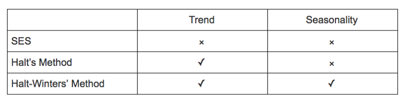
总结了指数平滑方法中不同分量形式的平滑参数。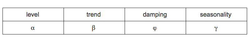
指数平滑是当今行业中应用最广泛、最成功的预测方法之一。如何预测零售额、游客数量、电力需求或收入增长?指数平滑是你需要展现未来的超能力之一。

若有收获,就点个赞吧
0 人点赞
