https://colab.research.google.com/drive/1EdgZaTb8mtc4vEnedNNtRygZ_Ls-jQqy?usp=sharing
边缘预测;
怎么把边分为train,val,test三个部分
使用PyG实现LightGCN
介绍
欢迎!在本文中,我们将学习如何使用图神经网络在 Spotify Million Playlist Dataset Challenge [1] 上执行音乐推荐。该数据集包含 2010 年 1 月至 2017 年 10 月期间用户在 Spotify 平台上创建的 100 万个播放列表。我们将使用该数据集的一个子集,因为它非常大。
我们的目标是推荐应该添加到每个播放列表的歌曲。我们将使用的主要指标是recall@k,它为每个播放列表计算如下: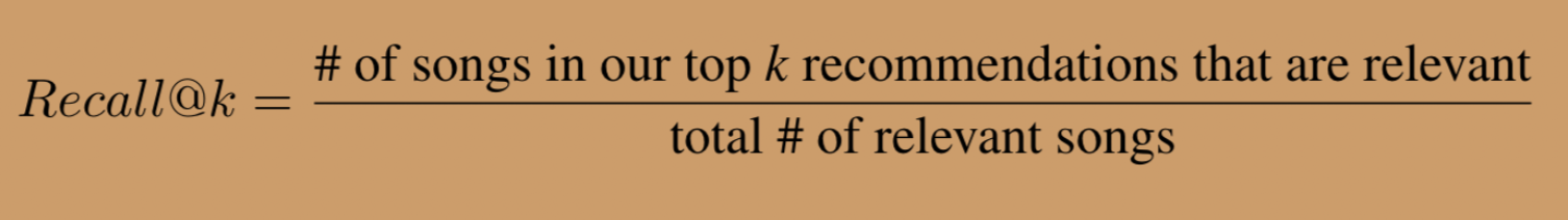
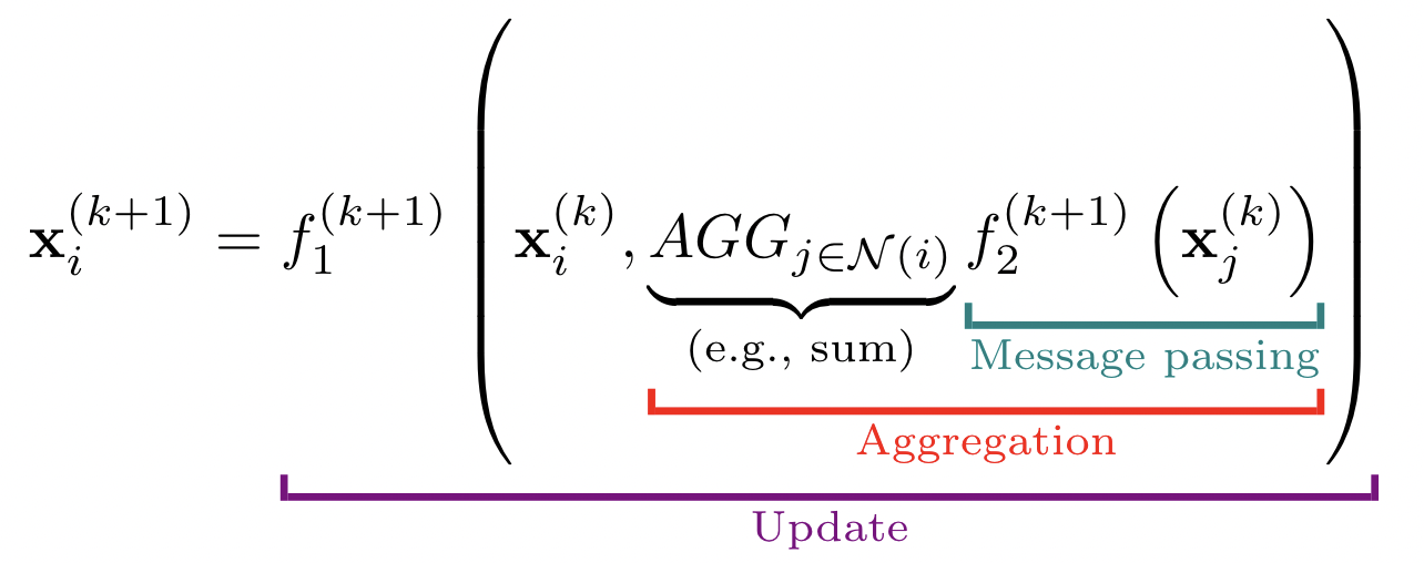 其中 f1 和 f2 是可微函数(通常是矩阵乘法与学习的权重矩阵),N(i) 是节点i的邻居,AGG 是聚合函数,例如 sum、mean 或 max。
最后一层 K 之后的节点嵌入可以用作特征来进行预测。在我们的例子中,我们想要预测一首歌曲是否属于一个播放列表,即预测两个节点之间是否存在一条边。为此,例如,我们可以将两个节点的嵌入连接在一起,并将它们通过一个小的密集层。或者,我们可以将两个节点的相似性定义为它们嵌入的点积。我们将使用第二个选项: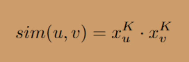
数据预处理
我们首先对数据进行预处理。我们将总结最重要的部分,但请在我们的GitHub 存储库中查看我们的预处理代码以获取更多详细信息。
Spotify 数据集有 100 万个播放列表、超过 200 万首独特的歌曲,以及超过 6600 万条将播放列表链接到歌曲的边。这是非常大的!我们将减少数据集,以便可以在合理的时间内在 Colab 上对其进行训练。为此,我们将计算图表的“K-core”。图 G 的 K 核是 G 的最大可能连通子图,其中每个节点的度至少为 K。这将给我们最大的子图,其中每个播放列表至少包含 K 首歌曲,并且每首歌曲是在至少 K 个播放列表中。
这有两个好处。首先,它将减少我们数据集的大小。其次,它将消除稀有/不受欢迎的歌曲和小型播放列表。其余的播放列表/歌曲都将是相对丰富的信息,这将使学习过程更容易一些,这对于本文的目的来说是理想的。
为了实际计算 K 核子图,我们将使用由 Jure Leskovec 教授领导的斯坦福大学 SNAP 小组的 SNAP 库。以计算 K=50 的 K-core 图为例,使用以下代码:
import snapG = snap.TUNGraph().New() # creates a new undirected graph... # add all nodes and edges to G (see SNAP docs or our full code for details)K = 50kcore = G.GetKCore(K)
训练/验证/测试拆分
评估任何 ML 问题的一个关键组成部分是训练/验证/测试拆分。这在 Graph ML 问题中尤为重要,在诸如此类的边缘/链接预测任务中更为重要。
为什么?在图中,数据点是高度相互关联和依赖的。例如,图像分类要容易得多;图像是独立的,因此我们可以简单地将每个图像分配给其中一个分割。有了图表,情况就不同了。如果节点 1 和节点 2 通过边连接,那么如果我们将节点 1 分配给测试集(并且不再在其上训练),那么这将影响我们对节点 2 的预测,因为节点 1 将用于消息传递到节点 2。
对于像我们这样的边缘预测任务,我们按边缘而不是节点进行分割。基本思想是在训练时隐藏一些边,将剩余的图作为输入传递给 GNN,然后在隐藏的边上进行预测。
因此,我们需要两种类型的边:1. 消息传递边,用于执行 GNN 传播,以及 2. 监督/评估边,用于计算损失和/或评估指标。
但我们还需要将这两组拆分为 train/val/test。这很棘手,不同的论文通常以不同的方式进行。然而,一种常见的方法是将边分成四组:训练消息边、训练监督边、验证边和测试边。然后:
- 在训练过程中,我们使用训练消息边来预测训练监督边,并计算损失。
- 在验证期间,我们使用训练消息边和训练监督边来预测验证边。
- 在测试期间,我们使用训练消息边、训练监督边和验证边来预测测试边。如下图所示:
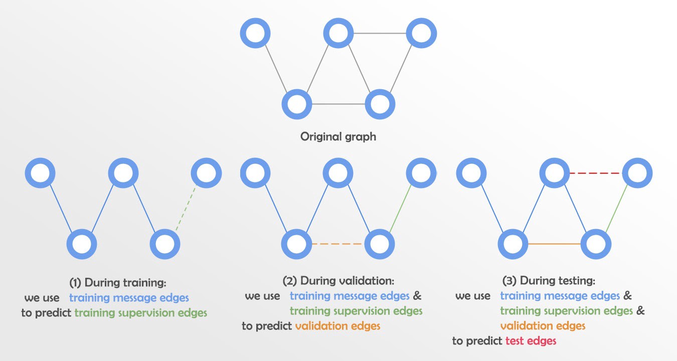
从技术上讲,我们将使用与训练监督边相同的训练消息传递边,这也是常见的做法。)
幸运的是,PyG 可以使用RandomLinkSplit为我们执行这种拆分!我们将使用 70%-15%-15% 的拆分。
from torch_geometric.transforms import RandomLinkSplittransform = RandomLinkSplit(is_undirected=True, add_negative_train_samples=False,neg_sampling_ratio=0, num_val=0.15, num_test=0.15)train_split, val_split, test_split = transform(data)
通过设置is_undirected=True,我们保证split之间不会有后向边的数据泄露(即边[2,4]和[4,2]应该在同一个split中,因为它们是同一个边,只是在相反的方向)。我们还设置 add_negative_train_samples=False 和 neg_sampling_ratio=0 以关闭所有三个拆分的负采样,因为我们将编写自己的负采样函数。
最后,我们将消息传递拆分存储在 PyG Data 对象中,并将监督/评估拆分存储在 PyG Dataset对象中,这将允许我们使用DataLoader批量加载它们。(有关更多详细信息,请参阅 Colab)。
有关图表上的训练/验证/测试拆分的更多信息,请参阅这些幻灯片。
使用PyG实现LightGCN
class LightGCN(MessagePassing):"""A single LightGCN layer. Extends the MessagePassing class from PyTorch Geometric"""def __init__(self):super(LightGCN, self).__init__(aggr='add') # aggregation function is 'add'def message(self, x_j, norm):"""Specifies how to perform message passing during GNN propagation. For LightGCN, we simply pass along eachsource node's embedding to the target node, normalized by the normalization term for that node.args:x_j: node embeddings of the neighbor nodes, which will be passed to the central node (shape: [E, emb_dim])norm: the normalization terms we calculated in forward() and passed into propagate()returns:messages from neighboring nodes j to central node i指定在GNN传播过程中如何进行消息传递。对于LightGCN,我们只是将每个源节点的嵌入传递给目标节点,并通过该节点的规范化项进行规范化处理。args:x_j:邻近节点的节点嵌入,将被传递给中心节点(形状:[E, emb_dim])norm:我们在forward()中计算的归一化项,并传递给propagate()。returns:从邻居节点j到中心节点i的信息"""# Here we are just multiplying the x_j's by the normalization terms (using some broadcasting)# 这里我们只是将x_j乘以归一化项(使用一些广播)。return norm.view(-1, 1) * x_jdef forward(self, x, edge_index):"""Performs the LightGCN message passing/aggregation/update to get updated node embeddingsargs:x: current node embeddings (shape: [N, emb_dim])edge_index: message passing edges (shape: [2, E])returns:updated embeddings after this layer执行LightGCN消息传递/聚合/更新,以获得更新的节点嵌入。args:x:当前节点嵌入(形状:[N, emb_dim])。edge_index:消息传递的边缘(形状:[2, E])。returns:本层之后的最新嵌入信息"""# Computing node degrees for normalization term in LightGCN (see LightGCN paper for details on this normalization term)# These will be used during message passing, to normalize each neighbor's embedding before passing it as a message# 计算LightGCN中归一化术语的节点度(关于这个归一化术语的细节,见LightGCN论文)# 这些将在消息传递过程中使用,在作为消息传递之前对每个邻居的嵌入进行标准化处理row, col = edge_indexdeg = degree(col)deg_inv_sqrt = deg.pow(-0.5)norm = deg_inv_sqrt[row] * deg_inv_sqrt[col]# Begin propagation. Will perform message passing and aggregation and return updated node embeddings.return self.propagate(edge_index, x=x, norm=norm)
希望上面的代码相当简单;我们在forward()中计算归一化项,将它们传递给propagate(),使用它们对message()中的每条消息x_j进行归一化,然后propagate()在内部处理聚合。现在,通过运行 forward(),我们在 LightGCN 层之后获得了更新的嵌入!
注意:请记住,除了用户/项目嵌入之外,LightGCN 没有任何可学习的权重矩阵。但是,对于确实使用这些的其他模型,我们可以很容易地添加一个 nn.Linear 层。例如,这里是 PyG 的 GCN_Conv 实现的源代码(链接)。
接下来,我们需要创建主要的 GNN 类,它将使用我们刚刚定义的 LightGCN 层。
完整代码
完整代码如下所示。在不解释每个细节的情况下,这里有几个关键点:
- 在构造函数中,我们初始化一个 nn.Embedding() 对象来存储我们的播放列表和歌曲的学习嵌入。此外,我们初始化了一个 LightGCN 层列表,我们将在传播过程中使用这些层。
- gnn_propagation() 在消息传递边上执行传播,以计算多尺度嵌入。它首先将第 0 层嵌入存储在一个列表中。然后它在每个 LightGCN 层传播,并将更新的嵌入附加到每个层的列表中。最后,取每层嵌入的平均值(即列表中的嵌入)来获得最终的多尺度嵌入。
- calc_loss() 是主要的训练函数。它首先调用 gnn_propagation() 来获取多尺度嵌入。然后它调用 predict_scores() 来获取正边缘和负边缘的分数。最后,它使用贝叶斯个性化排名(BPR)损失计算正/负边缘分数的损失,这是推荐问题的常见损失函数。
evaluation() 是主要的测试/评估功能。它找到每个播放列表的前 k 个推荐,然后计算召回率@k。remember_at_k() 是我们编写的辅助函数,您可以在我们的 Colab 中看到。
class GNN(torch.nn.Module):"""Overall GNN. Consists of learnable playlist/song embeddings and LightGCN layers."""def __init__(self, embedding_dim, num_nodes, num_playlists, num_layers):super(GNN, self).__init__()self.embedding_dim = embedding_dimself.num_nodes = num_nodes # total # of nodes (songs + playlists) in datasetself.num_playlists = num_playlists # total # of playlists in datasetself.num_layers = num_layers# Initialize embeddings for all playlists and songs. Playlists will have indices from# 0...num_playlists-1, songs will have indices from num_playlists...num_nodes-1self.embeddings = torch.nn.Embedding(num_embeddings=self.num_nodes, embedding_dim=self.embedding_dim)torch.nn.init.normal_(self.embeddings.weight, std=0.1)self.layers = torch.nn.ModuleList() # LightGCN layersfor _ in range(self.num_layers):self.layers.append(LightGCN())self.sigmoid = torch.sigmoiddef gnn_propagation(self, edge_index_mp):"""Performs linear embedding propagation and calculates final multi-scale embeddingsfor each user/item, which are calculated as the average of that user/item's embeddingsat each layer (from 0 to self.num_layers)args:edge_index_mp: tensor of all (undirected) edges in the graph, used for message passing/propagationand calculating multi-scale embeddings. (In contrast to evaluation/supervision edges, which arefor loss/performance metrics).returns:final multi-scale embeddings for all users/items"""x = self.embeddings.weight # layer-0 embeddingsx_at_each_layer = [x] # store embeddings from each layer. Start with layer-0 embeddingsfor i in range(self.num_layers): # now performing the GNN propagationx = self.layers[i](x, edge_index_mp)x_at_each_layer.append(x)final_embs = torch.stack(x_at_each_layer, dim=0).mean(dim=0) # take average to calculate multi-scale embeddingsreturn final_embsdef predict_scores(self, edge_index, embs):"""Calculate predicted score (using dot product) for each playlist/song pair in edge_indexargs:edge_index: tensor of edges (between playlists and songs) whose scores we will calculate.embs: node embeddings for calculating predicted scoresreturns:predicted scores for each playlist/song pair in edge_index"""scores = embs[edge_index[0,:], :] * embs[edge_index[1,:], :] # dot product for each playlist/song pairscores = scores.sum(dim=1)scores = self.sigmoid(scores)return scoresdef calc_loss(self, data_mp, data_pos, data_neg):"""Main training step. Performs GNN propagation on message passing edges, to get multi-scaleembeddings. Then predicts scores for each training example, and calculates BPR loss.args:data_mp: tensor of edges for message passing / calculating multi-scale embeddingsdata_pos: set of positive edges that will be used during loss calculationdata_neg: set of negative edges that will be used during loss calculationreturns:loss calculated on the positive/negative training edges"""# Perform GNN propagation on message passing edges to get final embeddingsfinal_embs = self.gnn_propagation(data_mp.edge_index)# Get edge prediction scores for all positive and negative evaluation edgespos_scores = self.predict_scores(data_pos.edge_index, final_embs)neg_scores = self.predict_scores(data_neg.edge_index, final_embs)# Calculate Bayesian Personalized Ranking loss (similar to the implementation used in# official LightGCN implementation at https://github.com/gusye1234/LightGCN-PyTorch)loss = -torch.log(self.sigmoid(pos_scores - neg_scores)).mean()return lossdef evaluation(self, data_mp, data_pos, k):"""Performs evaluation on validation or test set. Calculates recall@k.args:data_mp: message passing edges for propagation/calculating multi-scale embeddingsdata_pos: positive edges for scoring metrics. Should be no overlap with data_mpk: value of k to use for recall@kreturns:dictionary mapping playlist ID -> recall@k on that playlist"""# Run propagation on the message-passing edges to get multi-scale embeddingsfinal_embs = self.gnn_propagation(data_mp.edge_index)# Get embeddings of all unique playlists in the batch of evaluation edgesunique_playlists = torch.unique_consecutive(data_pos.edge_index[0,:])playlist_emb = final_embs[unique_playlists, :] # has shape [number of playlists in batch, 64]# Get embeddings of ALL songs in datasetsong_emb = final_embs[self.num_playlists:, :] # has shape [total number of songs in dataset, 64]# All ratings for each playlist in batch to each song in entire dataset (using dot product as the scoring function)ratings = self.sigmoid(torch.matmul(playlist_emb, song_emb.t())) # shape: [# playlists in batch, # songs in dataset]# where entry i,j is rating of song j for playlist i# Calculate recall@kresult = recall_at_k(ratings.cpu(), k, self.num_playlists, data_pos.edge_index.cpu(),unique_playlists.cpu(), data_mp.edge_index.cpu())return result
为简洁起见,我们将省略 train() 和 test() 循环的代码,但它们在 Colab 中可用。train() 循环的主要独特部分是它执行一些负采样(为每个播放列表获取负歌曲,即不在播放列表中的歌曲),以便我们可以计算 BPR 损失。我们的负采样功能在 Colab 中也是可见的。
训练
现在我们准备好训练了,看看我们的模型是怎么做的!
在 Colab 数据集中,大约有 5,700 首独特的歌曲。因此,对于本文,我们为recall@k 设置k=300。这似乎是合理的,因为这意味着我们希望模型在 5700 首歌曲中预测前 300 首歌曲中的正确歌曲,这大约是前 5%。当然,您可以随意使用不同的值,甚至可以使用多个值并取平均值。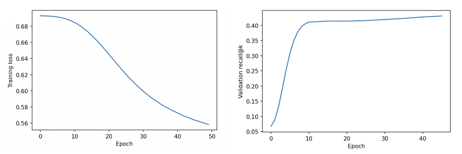
可视化学习的嵌入(使用动画!)
现在我们已经完成了模型的训练,让我们对我们学习的嵌入进行一些分析。看看不同的歌曲和播放列表在高维空间中映射到哪里会很有趣!
请查看 Colab 获取完整代码,并重新创建这些 GIF!
向下投影到二维
我们的嵌入是 64 维的,太大而无法可视化。因此,我们使用 Scikit-Learn (链接) 中的主成分分析 (PCA) 实现将我们所有的播放列表/歌曲嵌入投影到二维,以便我们可以在二维中绘制它们。
第 1 步:分析乡村音乐播放列表
在检查嵌入时,我们注意到有一组不同的播放列表似乎与其他播放列表分开。在对这些数据点进行了一些手动检查后,我们意识到它们主要是乡村音乐播放列表。
因此,我们编写了一些代码来查找标题中包含“国家”一词的所有播放列表。虽然不是一个完美的方法,但这是查找国家/地区播放列表的良好代理。我们发现在 9296 个播放列表中,有 736 个是乡村音乐。
接下来,我们制作了一个动画 GIF(您也可以在 Colab 中重新创建),以红色绘制国家播放列表,以蓝色绘制所有其他播放列表。它是动画的,因为我们展示了前 10 个时期的进展。一开始,嵌入大多是随机的,这是有道理的。但到最后,我们可以看到模型自动检测到的乡村音乐播放列表的清晰集群!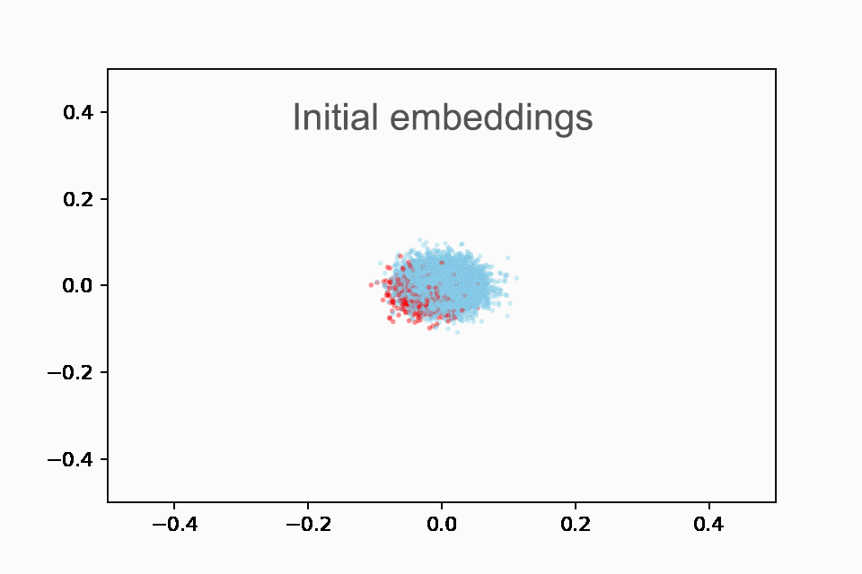
在训练的前 10 个时期内显示乡村音乐播放列表(红色)与非乡村音乐播放列表(蓝色)嵌入的动画。在开始时(纪元 0),所有播放列表都聚集在中心。到最后(第 10 纪元),国家和非国家播放列表之间有明显的区别。
第 2 步:分析 Drake 歌曲
接下来,除了播放列表之外,我们还想可视化一些歌曲。Drake 是我们数据集中最受欢迎的艺术家之一,在我们的数据集中有 118 首歌曲。我们再次制作了一个 GIF 来绘制 Drake 歌曲在前 10 个时期的嵌入。
再次,您可以看到,虽然所有的嵌入都以一个大簇开始,但到最后,Drake 的歌曲(红色)显然已经开始聚集在同一个区域!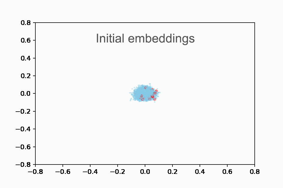
在训练的前 10 个时期内,动画显示了 Drake 歌曲(红色)与所有其他歌曲(蓝色)的嵌入。一开始,所有歌曲都聚集在中心。到最后,Drake 的歌曲都清楚地聚集在嵌入空间的同一个一般区域中。
第 3 步:分析 Taylor Swift 的歌曲
我们将最有趣的发现留到最后。我们首先重新创建了与 Drake 相同的动画,如下所示: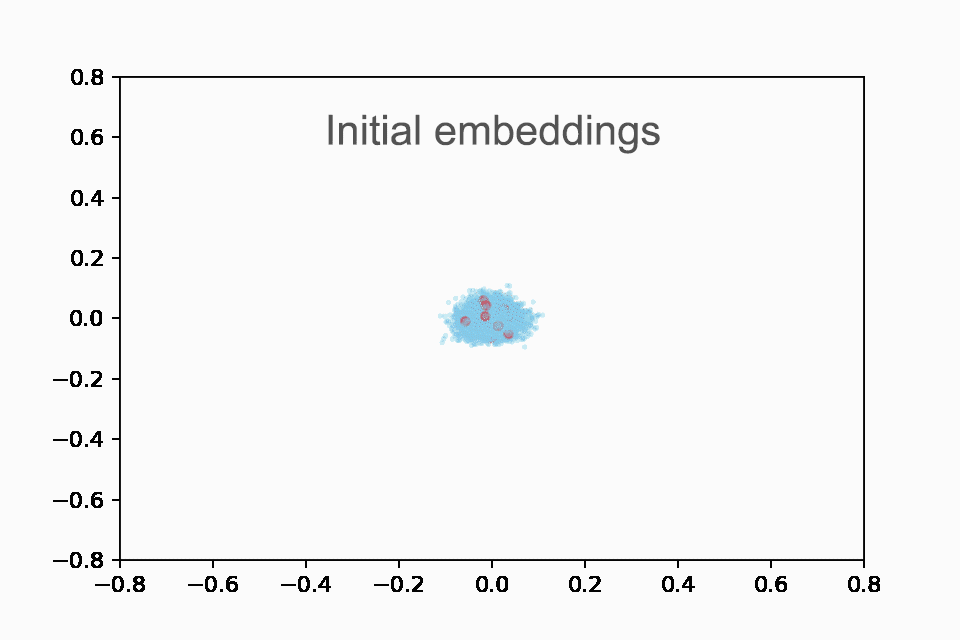
在训练的前 10 个 epoch 中显示 Taylor Swift 歌曲(红色)与所有其他歌曲(蓝色)的嵌入的动画。
您可能会注意到一些非常有趣的事情!在 GIF 的结尾处,Taylor Swift 的歌曲正好在中间,处于乡村歌曲与非乡村歌曲之间的边界。这实际上很有意义,因为她最初是一名乡村歌手,后来转向流行音乐。
(细心的读者注意:我们现在绘制的是歌曲而不是播放列表,所以不清楚这个 GIF 中的集群是否也是乡村歌曲。但是,我们可以确认它是,既来自我们自己的检查,也因为它就模型而言是有意义的。由于我们通过歌曲和播放列表之间的点积来计算分数,因此国家播放列表和国家歌曲具有相似的嵌入是有意义的,因为这将使点积最大化。所以它们很可能都嵌入在相似的位置)。
为了进一步探索这些泰勒斯威夫特的结果,我们决定手动将泰勒斯威夫特的 21 首歌曲中的每一首歌曲分类为来自她职业生涯的乡村音乐和流行音乐阶段。我们这样做主要是基于她在维基百科上的歌曲描述。(有关我们的分类,请参阅 Colab)。我们现在在 epoch 10 之后再次绘制嵌入,她的乡村歌曲为蓝色,她的流行歌曲为红色,所有其他歌曲为灰色。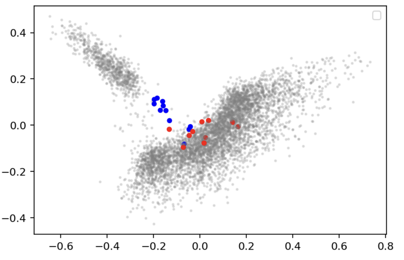
在 Epoch 10 之后,Taylor Swift 的乡村歌曲(蓝色)与她的流行歌曲(红色)的嵌入。所有其他歌曲都是灰色的。左上角的灰色集群主要是乡村歌曲,因此她的乡村歌曲(蓝色)比她的流行歌曲更接近该集群是有道理的。模特已经学会了自己识别她职业生涯的两半!
看来我们的猜测是正确的!她的乡村(蓝色)歌曲更接近乡村歌曲集群,而她的流行(红色)歌曲更接近非乡村歌曲集群。
这是一个非常有趣的结果。我们的模型似乎已经学会了将泰勒斯威夫特职业生涯的不同阶段完全独立地嵌入到两个部分中!
结论
我们希望本文能帮助您了解图神经网络的强大功能,并了解如何自己实现它们。有许多有趣的图问题需要探索,像 PyG 这样的工具使这比以往任何时候都更容易做到。
在我们的数据集上,我们在召回@k 等指标方面取得了良好的表现。我们还分析了嵌入本身,发现它们能够区分国家和非国家播放列表,将 Drake 的所有歌曲聚集在同一个大区,甚至区分泰勒斯威夫特早期的乡村生涯和她后来的流行生涯,没有任何额外的人工监督!
如需更多信息,我们强烈建议您查看斯坦福大学CS224W的课程资料。

若有收获,就点个赞吧
0 人点赞
