Medium链接:https://youyoung-jang.medium.com/exploring-pytorch-geometric-with-reddit-data-b38a9a44eec0
Exploring Pytorch Geometric with Reddit Dataset
图同构网络Graph Isomorphism Network 是一种强大且富有表现力的算法,可在 GNN 之间实现最大的判别力。尽管它很简单,但它显示出很强的代表性。
在本文中,我将向您展示如何使用 Pytorch Geometric 的核心组件并通过邻居采样实现图同构网络的示例。
Reddit 数据
您可以使用以下代码轻松下载数据集。
os.getcwd() 方法用于返回当前工作目录。
print(os.path.join(‘root’,’test’,’runoob.txt’))# 将目录和文件名合成一个路径
root/test/runoob.txt
import osfrom torch_geometric.datasets import Reddit# Load Reddit Datasetpath = os.path.join(os.getcwd(), 'data', 'Reddit')dataset = Reddit(path)data = dataset[0]
如果同一用户对两个帖子发表了评论,则两个帖子之间存在链接。这些帖子属于某个社区。数据中包含 41 个社区,任务是预测帖子属于哪个社区。
查看下面的代码。
# Nodes: 232965, Node Features: 602, Edge Index: (2, 114M)num_communities = len(set(data.y.numpy().tolist()))print(f"Node Feature Matrix Info: # Nodes: {data.x.shape[0]}")print(f"Node Feature Matrix Info: # Node Features: {data.x.shape[1]}")print(f"Edge Index Shape: {data.edge_index.shape}")print(f"Edge Weight: {data.edge_attr}")print(f"# Community: {num_communities}")# you can also check additional informationprint(data.contains_isolated_nodes())print(data.contains_self_loops())print(data.is_directed())
邻居采样器
当全批训练不是最佳方法时,有几种方法可以配置输入数据。值得庆幸的是,Pytorch Geometric 支持各种工具来处理大图数据。邻居采样器就是其中之一。
Neighbor Sampler 允许您使用小批量设置训练大规模图形。因为它对一组固定大小的邻居进行采样,这可能导致梯度估计不太准确。但是,当您遇到巨大的图表时,这仍然是一个有用的选项。如果您想了解更多详细信息,请在此处查看官方文档。
现在让我们为 Reddit 数据创建邻居采样器。
# Create Neighbor samplernum_samples = [10, 5]num_layers = len(num_samples)train_neigh_sampler = NeighborSampler(data.edge_index, node_idx=data.train_mask+data.val_mask,sizes=num_samples, batch_size=1024, shuffle=True, num_workers=0)subgraph_loader = NeighborSampler(data.edge_index, node_idx=None,sizes=[-1], batch_size=1024, shuffle=False, num_workers=0)
您可以num_samples通过sizes参数提供。上面的示例显示,您为 1 跳邻居采样 10 个节点,为 2 跳邻居采样 5 个节点。这意味着每个头节点有 50 个节点。
如果您将这些数字设置得太小,那么您的模型可能无法通过邻居采样捕获足够的信息。另一方面,如果你把这些数字设置得太大,那么训练模型的速度就会变慢,而且你可能会遇到过度平滑的问题。所以你应该找到合适的采样节点数。
一下子搞清楚 Reddit 数据和 Neighbor Sampler 的结构并不容易。让我们一步一步来了解。
Neighbor Sampler 的输出如下。
batch_size, n_id, adjs = next(iter(train_neigh_sampler))
batch_size只是批量大小整数。n_id包含当前批次中出现的所有节点 ID。例如,n_id可以是长度为 45677 的张量。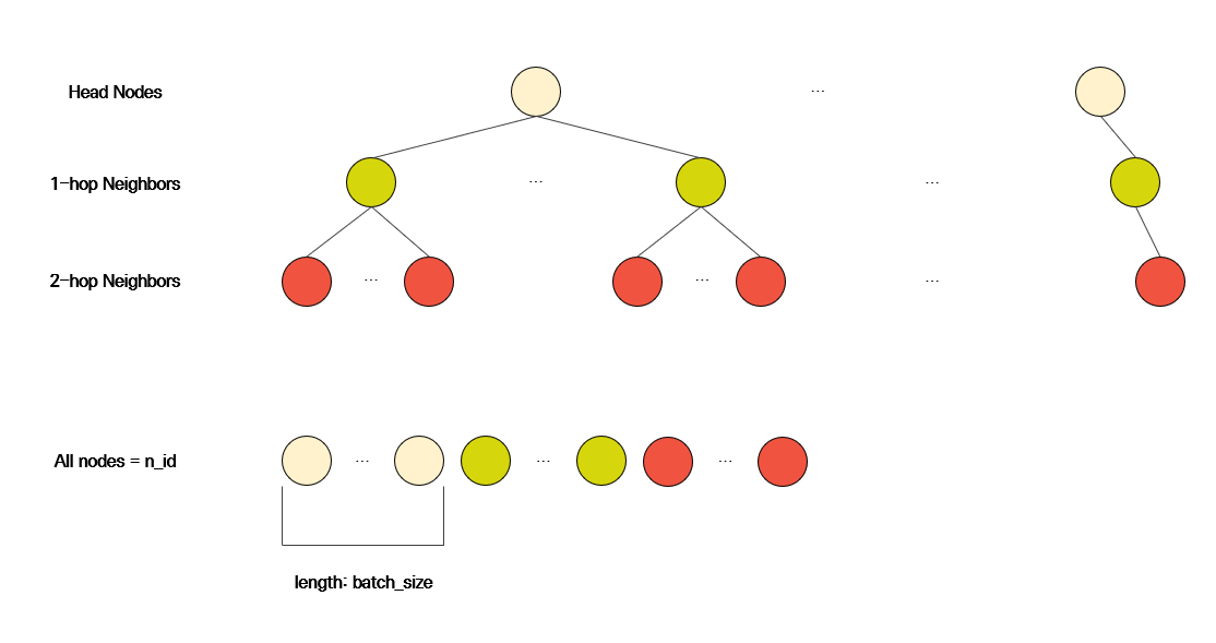
邻居抽样过程
请注意,最后一行中圆圈数的总和等于n_id 的长度,并且节点 ID 按采样步骤排序。所以头节点总是排在第一位的。您可以利用这一事实创建批处理数据。
device = torch.device('cuda' if torch.cuda.is_available() else 'cpu')X = data.x.to(device)Y = data.y.squeeze().to(device)batch_size, n_id, adjs = next(iter(train_neigh_sampler))adjs = [adj.to(device) for adj in adjs]x_batch = X[n_id]y_batch = Y[n_id[:batch_size]]
现在让我们看一下adjs部分。因为我们选择使用 2 层,所以adjs列表的长度为 2。在这个例子adjs[1]中,表达了头节点和 1-hop 邻居之间的关系,并adjs[0]包含 1-hop 邻居和 2-hop 邻居之间的信息。您应该记住,顺序是相反的,因为源节点的特征会传播到目标节点的特征。
首先,让我们看一下adjs[1]部分。
edge_index, e_id, size = adjs[1]
edge_index的格式与data.edge_index的格式相同,但edge_index中的节点 id已根据子图结构重新索引。e_id包含 edge_index中使用的原始节点 ID。size是一个元组,表示 edge_index中的节点数。
例如,假设 1 跳邻居的数量为 A,2 跳邻居的数量为 B。那么大小为(A+B, A)。
带采样的图同构网络
# Define Modelfrom torch.nn import Sequential, Linear, BatchNorm1d, ReLU, Dropoutfrom torch_geometric.nn import GINConvclass GIN(torch.nn.Module):def __init__(self, drop_rate, num_node_features, num_layers, hidden_size, out_channels):super(GIN, self).__init__()self.drop_rate = drop_rateself.num_node_features = num_node_featuresself.num_layers = num_layersself.hidden_size = hidden_sizeself.out_channels = out_channelsself.gin_convs = torch.nn.ModuleList()self.gin_convs.append(GINConv(nn=Sequential(Linear(in_features=num_node_features, out_features=hidden_size),BatchNorm1d(num_features=hidden_size),ReLU(),Dropout(p=drop_rate),Linear(hidden_size, hidden_size),ReLU())))self.gin_convs.append(GINConv(nn=Sequential(Linear(in_features=hidden_size, out_features=hidden_size),BatchNorm1d(num_features=hidden_size),ReLU(),Dropout(p=drop_rate),Linear(hidden_size, out_channels))))def forward(self, x_batch, adjs):# x_batch = X[n_id] or data.x[n_id]# x_batch = head_node_features + 1_hop_node_features + 2_hop_node_featuresfor i, (edge_index, e_id, size) in enumerate(adjs):# size ex) (10399, 1024) or (45887, 10399)x_target = x_batch[:size[1]]x_batch = self.gin_convs[i]((x_batch, x_target), edge_index)out = F.log_softmax(x_batch, dim=-1)return outdef inference(self, x_all):pbar = tqdm(total=x_all.size(0) * self.num_layers)pbar.set_description('Testing')for i in range(self.num_layers):xs = []for batch_size, n_id, adj in subgraph_loader:edge_index, _, size = adj.to(device)x = x_all[n_id].to(device)x_target = x[:size[1]]x = self.gin_convs[i]((x, x_target), edge_index)if i != self.num_layers - 1:x = F.relu(x)xs.append(x.cpu())pbar.update(batch_size)x_all = torch.cat(xs, dim=0)pbar.close()return x_alldevice = torch.device('cuda' if torch.cuda.is_available() else 'cpu')model = GIN(drop_rate=0.2, num_node_features=data.num_node_features, num_layers=num_layers,hidden_size=128, out_channels=num_communities)model = model.to(device)optimizer = torch.optim.Adam(model.parameters(), lr=0.01)X = data.x.to(device)Y = data.y.squeeze().to(device)
您可以随时更改模型结构以提高性能。GIN 可以很容易地使用GINConv. 在此示例中,我设置hidden_size为 128 和drop_rate0.2 和num_communities41,因为 Reddit 数据中有 41 个社区。
现在让我们使用以下代码训练模型
def train(epoch):model.train()pbar = tqdm(total=int(data.train_mask.sum()))pbar.set_description(f'Epoch {epoch:02d}')total_loss = total_correct = 0for batch_size, n_id, adjs in train_neigh_sampler:adjs = [adj.to(device) for adj in adjs]optimizer.zero_grad()out = model(X[n_id], adjs)loss = F.nll_loss(out, Y[n_id[:batch_size]])loss.backward()optimizer.step()total_loss += float(loss)total_correct += int(out.argmax(dim=-1).eq(Y[n_id[:batch_size]]).sum())pbar.update(batch_size)pbar.close()loss = total_loss / len(train_neigh_sampler)approx_acc = total_correct / int(data.train_mask.sum()+data.val_mask.sum())return loss, approx_acc@torch.no_grad()def test():model.eval()out = model.inference(X)y_true = Y.cpu().unsqueeze(-1)y_pred = out.argmax(dim=-1, keepdim=True)results = []for mask in [data.train_mask+data.val_mask, data.test_mask]:results += [int(y_pred[mask].eq(y_true[mask]).sum()) / int(mask.sum())]return resultsfor epoch in range(1, 21):loss, acc = train(epoch)print(f'Epoch {epoch:02d}, Loss: {loss:.4f}, Approx. Train: {acc:.4f}')train_acc, test_acc = test()print(f'Train: {train_acc:.4f}, Test: {test_acc:.4f}')
20个Epochs后,结果如下。
损失:0.3046,训练 Acc:0.8916,测试 ACC:0.8949
我的实验是在配备 NVIDIA GeForce RTX 3070 Ti(8GB 内存)、6 核 AMD Ryzen 5 5600X CPU(3.70 GHz)和 24 GB RAM 的机器上进行的。
更新于 2021 年 8 月 16 日

若有收获,就点个赞吧
0 人点赞
