获取数据

数据集包括了 2013 年 9 月份两天时间内的信用卡交易数据，284807 笔交易中，一共有 492 笔是欺诈行为。输入数据一共包括了 28 个特征 V1，V2，……V28 对应的取值，以及交易时间 Time 和交易金额 Amount。为了保护数据隐私，我们不知道 V1 到 V28 这些特征代表的具体含义，只知道这 28 个特征值是通过 PCA 变换得到的结果。另外字段 Class 代表该笔交易的分类，Class=0 为正常（非欺诈），Class=1 代表欺诈。针对这个数据集构建一个信用卡欺诈分析的分类器，并计算F1。

import pandas as pd
import numpy as np
from sklearn.linear_model import LogisticRegression
from sklearn.model_selection import train_test_split
from sklearn.preprocessing import StandardScaler
from sklearn.metrics import recall_score,roc_curve,confusion_matrix#召回率，精准率，混合矩阵
import warnings 
warnings.filterwarnings('ignore')
import matplotlib.pyplot as plt
import seaborn as sns
plt.rcParams['font.sans-serif']=['Heiti TC']# 显示中文字体

data=pd.read_csv('creditcard.csv')

数据探索

data.head()

5 rows × 31 columns

data.info()

<class 'pandas.core.frame.DataFrame'>
RangeIndex: 284807 entries, 0 to 284806
Data columns (total 31 columns):
Time      284807 non-null float64
V1        284807 non-null float64
V2        284807 non-null float64
V3        284807 non-null float64
V4        284807 non-null float64
V5        284807 non-null float64
V6        284807 non-null float64
V7        284807 non-null float64
V8        284807 non-null float64
V9        284807 non-null float64
V10       284807 non-null float64
V11       284807 non-null float64
V12       284807 non-null float64
V13       284807 non-null float64
V14       284807 non-null float64
V15       284807 non-null float64
V16       284807 non-null float64
V17       284807 non-null float64
V18       284807 non-null float64
V19       284807 non-null float64
V20       284807 non-null float64
V21       284807 non-null float64
V22       284807 non-null float64
V23       284807 non-null float64
V24       284807 non-null float64
V25       284807 non-null float64
V26       284807 non-null float64
V27       284807 non-null float64
V28       284807 non-null float64
Amount    284807 non-null float64
Class     284807 non-null int64
dtypes: float64(30), int64(1)
memory usage: 67.4 MB

data.describe()

8 rows × 31 columns

# 欺诈和正常交易可视化
f, (ax1, ax2) = plt.subplots(2, 1, sharex=True, figsize=(15,8))
bins = 50
ax1.hist(data.Time[data.Class == 1], bins = bins, color = 'deeppink')
ax1.set_title('诈骗交易')
ax2.hist(data.Time[data.Class == 0], bins = bins, color = 'deepskyblue')
ax2.set_title('正常交易')
plt.xlabel('时间')
plt.ylabel('交易次数')
plt.show()

清洗数据

数据较为干净未发现缺失值

单变量分析

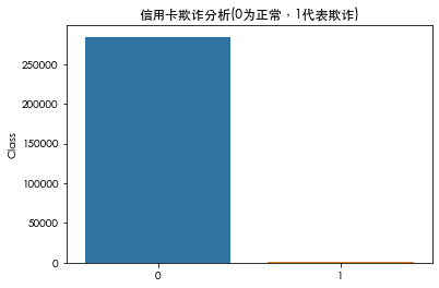
count=pd.DataFrame(data['Class'].value_counts())
sns.barplot(x=count.index,y=count['Class'])
plt.title('信用卡欺诈分析(0为正常，1代表欺诈)')
plt.show()

特征选取

data.corr()['Class'].sort_values()

V17      -0.326481
V14      -0.302544
V12      -0.260593
V10      -0.216883
V16      -0.196539
V3       -0.192961
V7       -0.187257
V18      -0.111485
V1       -0.101347
V9       -0.097733
V5       -0.094974
V6       -0.043643
Time     -0.012323
V24      -0.007221
V13      -0.004570
V15      -0.004223
V23      -0.002685
V22       0.000805
V25       0.003308
V26       0.004455
Amount    0.005632
V28       0.009536
V27       0.017580
V8        0.019875
V20       0.020090
V19       0.034783
V21       0.040413
V2        0.091289
V4        0.133447
V11       0.154876
Class     1.000000
Name: Class, dtype: float64

def remove_collinear_features(x, threshold):
    '''
    Objective:
       删除数据帧中相关系数大于阈值的共线特征。 删除共线特征可以帮助模型泛化并提高模型的可解释性。

    Inputs: 
        阈值：删除任何相关性大于此值的特征

    Output: 
        仅包含非高共线特征的数据帧
    '''

    y = x['Class']
    x = x.drop(columns = ['Class'])

    # 计算相关性矩阵
    corr_matrix = x.corr()
    iters = range(len(corr_matrix.columns) - 1)
    drop_cols = []

    # 迭代相关性矩阵并比较相关性
    for i in iters:
        for j in range(i):
            item = corr_matrix.iloc[j:(j+1), (i+1):(i+2)]
            col = item.columns
            row = item.index
            val = abs(item.values)

            # 如果相关性超过阈值
            if val >= threshold:
                # 打印有相关性的特征和相关值
                # print(col.values[0], "|", row.values[0], "|", round(val[0][0], 2))
                drop_cols.append(col.values[0])

    # 删除每对相关列中的一个
    drops = set(drop_cols)

    # 将得分添加回数据
    x['Class'] = y

    return x

# 删除相关性大于0.6的特征向量
features = remove_collinear_features(data, 0.6)

发现变量之前不存在互相影响的情况，针对V1-28进行研究

# 对金额进行标准化处理
data['Amount_Norm']=StandardScaler().fit_transform(data['Amount'].values.reshape(-1,1))

结果显示数据之间不存在共线性问题

构建模型

data['Amount_Norm'] = StandardScaler().fit_transform(data['Amount'].values.reshape(-1,1))
# 特征选择
y = np.array(data.Class.tolist())
data = data.drop(['Time','Amount','Class'],axis=1)
X = np.array(data.as_matrix())
# 准备训练集和测试集
train_x, test_x, train_y, test_y = train_test_split (X, y, test_size = 0.1, random_state = 33)

# 逻辑回归分类
clf = LogisticRegression()
clf.fit(train_x, train_y)
predict_y = clf.predict(test_x)

recall_score,roc_curve,confusion_matrix

#计算召回率
R=recall_score(predict_y,test_y)
print('召回率R='+str(R))

召回率R=0.8409090909090909

指标解释

fpr, tpr, thresholds=roc_curve(predict_y,test_y)
plt.plot(fpr,tpr,marker = 'o')
plt.ylabel('真阳性率 = true positive rate = TPR = TP/ (TP + FN)')
plt.xlabel("假阳性率 = false positive rate = FPR = FP / (FP+TN)")
plt.show()

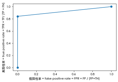
from sklearn.metrics import auc
AUC = auc(fpr, tpr)
print('AUC='+str(AUC))

AUC=0.9200501427397725

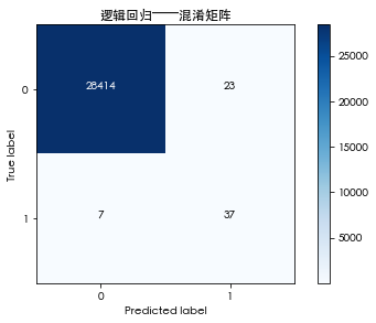
cm=confusion_matrix(predict_y,test_y,labels=[0,1])

import itertools
classes= [0,1]
cmap = plt.cm.Blues
plt.figure()
plt.imshow(cm, interpolation = 'nearest', cmap = cmap)
plt.title('逻辑回归——混淆矩阵')
plt.colorbar()
tick_marks = np.arange(len(classes))
plt.xticks(tick_marks, classes, rotation = 0)
plt.yticks(tick_marks, classes)

thresh = cm.max() / 2.
for i, j in itertools.product(range(cm.shape[0]), range(cm.shape[1])) :
    plt.text(j, i, cm[i, j],
             horizontalalignment = 'center',
             color = 'white' if cm[i, j] > thresh else 'black')

plt.tight_layout()
plt.ylabel('True label')
plt.xlabel('Predicted label')
plt.show()