- 1、介绍、安装、使用
- 2、quickstart
- 9 numbers from 0 to 2
- jy: array([0. , 0.25, 0.5 , 0.75, 1. , 1.25, 1.5 , 1.75, 2. ])
- useful to evaluate function at lots of points
- elementwise product
- matrix product
- another matrix product
- sum of each column
- min of each row
- cumulative sum along each row
- jy: array([ 0, 1, 8, 27, 64, 125, 216, 343, 512, 729])
- jy: 8
- jy: array([ 8, 27, 64])
- equivalent to a[0:6:2] = 1000;
- from start to position 6, exclusive, set every 2nd element to 1000
- jy: array([1000, 1, 1000, 27, 1000, 125, 216, 343, 512, 729])
- jy: array([ 729, 512, 343, 216, 125, 1000, 27, 1000, 1, 1000])
- the last row. Equivalent to b[-1, :]
- jy: array([40, 41, 42, 43])
- 3、Shape Manipulation
- jy: (3, 4)
- Split
ainto 3 - Split
aafter the third and the fourth column - id is a unique identifier of an object
- s[:] is a view of s. Note the difference between s = 10 and s[:] = 10
- 5、Broadcasting rules
- 6、Advanced indexing and index tricks
- the first 12 square numbers
- an array of indices
- the elements of
aat the positionsi - jy: array([ 1, 1, 9, 64, 25])
- a bidimensional array of indices
- the same shape as
j - indices for the first dim of
a - indices for the second dim
- i and j must have equal shape
- not what we want
- same as
a[i, j] - jy: array([0, 1, 2, 3, 4])
- jy: array([0, 0, 2, 0, 0])
bis a boolean witha‘s shape- 1d array with the selected elements
- jy: array([ 5, 6, 7, 8, 9, 10, 11])
- jy: array([[[5, 4, 6, 8, 3]]])
- jy: ((4, 1, 1), (1, 3, 1), (1, 1, 5))
- jy: 17
- jy: 17
- 7、Tricks and Tips
- jy: array([0, 2, 4, 6, 8, 0, 1, 2, 3, 4])
1、介绍、安装、使用
1)介绍
- NumPy is the fundamental package for scientific computing in Python. It is a Python library that provides a multidimensional array object, various derived objects (such as masked arrays and matrices), and an assortment of routines for fast operations on arrays, including mathematical, logical, shape manipulation, sorting, selecting, I/O, discrete Fourier transforms, basic linear algebra, basic statistical operations, random simulation and much more.
- At the core of the NumPy package, is the ndarray object. This encapsulates n-dimensional arrays of homogeneous data types, with many operations being performed in compiled code for performance.
- There are several important differences between NumPy arrays and the standard Python sequences:
- NumPy arrays have a fixed size at creation, unlike Python lists (which can grow dynamically). Changing the size of an ndarray will create a new array and delete the original.
- The elements in a NumPy array are all required to be of the same data type, and thus will be the same size in memory.
- The exception: one can have arrays of (Python, including NumPy) objects, thereby allowing for arrays of different sized elements.
- NumPy arrays facilitate advanced mathematical and other types of operations on large numbers of data. Typically, such operations are executed more efficiently and with less code than is possible using Python’s built-in sequences.
- A growing plethora([ˈpleθərə] 过多; 过量; 过剩)of scientific and mathematical Python-based packages are using NumPy arrays; though these typically support Python-sequence input, they convert such input to NumPy arrays prior to processing, and they often output NumPy arrays. In other words, in order to efficiently use much (perhaps even most) of today’s scientific/mathematical Python-based software, just knowing how to use Python’s built-in sequence types is insufficient - one also needs to know how to use NumPy arrays.
- The points about sequence size and speed are particularly important in scientific computing. As a simple example, consider the case of multiplying each element in a 1-D sequence with the corresponding element in another sequence of the same length.
If the data are stored in two Python lists,
aandb, we could iterate over each element:c = []for i in range(len(a)):c.append(a[i]*b[i])
This produces the correct answer, but if
aandbeach contain millions of numbers, we will pay the price for the inefficiencies of looping in Python. We could accomplish the same task much more quickly in C by writing (for clarity we neglect variable declarations and initializations, memory allocation, etc.)for (i = 0; i < rows; i++): {c[i] = a[i] * b[i];}
This saves all the overhead involved in interpreting the Python code and manipulating Python objects, but at the expense of the benefits gained from coding in Python. Furthermore, the coding work required increases with the dimensionality of our data.
In the case of a 2-D array, for example, the C code (abridged as before) expands to
for (i = 0; i < rows; i++): {for (j = 0; j < columns; j++): {c[i][j] = a[i][j] * b[i][j];}}
NumPy gives us the best of both worlds: element-by-element operations are the “default mode” when an ndarray is involved, but the element-by-element operation is speedily executed by pre-compiled C code.
In NumPy:
c = a * b
does what the earlier examples do, at near-C speeds, but with the code simplicity we expect from something based on Python. Indeed, the NumPy idiom is even simpler! This last example illustrates two of NumPy’s features which are the basis of much of its power: vectorization and broadcasting.
(a)Why is NumPy Fast?
Vectorization describes the absence of any explicit looping, indexing, etc., in the code - these things are taking place, of course, just “behind the scenes” in optimized, pre-compiled C code.
- Vectorized code has many advantages, among which are:
- vectorized code is more concise and easier to read
- fewer lines of code generally means fewer bugs
- the code more closely resembles standard mathematical notation (making it easier, typically, to correctly code mathematical constructs)
- vectorization results in more “Pythonic” code. Without vectorization, our code would be littered with inefficient and difficult to read for loops.
Broadcasting is the term used to describe the implicit element-by-element behavior of operations; generally speaking, in NumPy all operations, not just arithmetic operations, but logical, bit-wise, functional, etc., behave in this implicit element-by-element fashion, i.e., they broadcast. Moreover, in the example above,
aandbcould be multidimensional arrays of the same shape, or a scalar and an array, or even two arrays of with different shapes, provided that the smaller array is “expandable” to the shape of the larger in such a way that the resulting broadcast is unambiguous.- For detailed “rules” of broadcasting:
- https://numpy.org/doc/stable/user/basics.broadcasting.html#basics-broadcasting
(b)Who Else Uses NumPy?
- https://numpy.org/doc/stable/user/basics.broadcasting.html#basics-broadcasting
- For detailed “rules” of broadcasting:
NumPy fully supports an object-oriented approach, starting, once again, with ndarray. For example, ndarray is a class, possessing numerous methods and attributes. Many of its methods are mirrored by functions in the outer-most NumPy namespace, allowing the programmer to code in whichever paradigm they prefer. This flexibility has allowed the NumPy array dialect and NumPy ndarray class to become the de-facto language of multi-dimensional data interchange used in Python.
2)安装
-
2、quickstart
This is a quick overview of arrays in NumPy. It demonstrates how n-dimensional (n>=2) arrays are represented and can be manipulated.
Learning Objectives
NumPy’s main object is the homogeneous multidimensional array. It is a table of elements (usually numbers), all of the same type, indexed by a tuple of non-negative integers. In NumPy dimensions are called axes.
For example, the array for the coordinates of a point in 3D space,
[1, 2, 1], has one axis. That axis has 3 elements in it, so we say it has a length of 3. In the example pictured below, the array has 2 axes. The first axis has a length of 2, the second axis has a length of 3.[[1., 0., 0.],[0., 1., 2.]]
NumPy’s array class is called ndarray. It is also known by the alias array. Note that numpy.array is not the same as the Standard Python Library class array.array, which only handles one-dimensional arrays and offers less functionality. The more important attributes of an ndarray object are:
- ndarray.ndim
- the number of axes (dimensions) of the array.
- ndarray.shape
- the dimensions of the array. This is a tuple of integers indicating the size of the array in each dimension. For a matrix with
_n_rows and_m_columns,shapewill be(n,m). The length of theshapetuple is therefore the number of axes,ndim.
- the dimensions of the array. This is a tuple of integers indicating the size of the array in each dimension. For a matrix with
- ndarray.size
- the total number of elements of the array. This is equal to the product of the elements of shape.
- ndarray.dtype
- an object describing the type of the elements in the array. One can create or specify dtype’s using standard Python types. Additionally NumPy provides types of its own.
numpy.int32,numpy.int16, andnumpy.float64are some examples.
- an object describing the type of the elements in the array. One can create or specify dtype’s using standard Python types. Additionally NumPy provides types of its own.
- ndarray.itemsize
- the size in bytes of each element of the array.
- For example, an array of elements of type float64 has itemsize 8 (=64/8), while one of type complex32 has itemsize 4 (=32/8). It is equivalent to
ndarray.dtype.itemsize.
- ndarray.data
- the buffer containing the actual elements of the array. Normally, we won’t need to use this attribute because we will access the elements in an array using indexing facilities. ```python import numpy as np
- ndarray.ndim
a = np.arange(15).reshape(3, 5) print(a) “”” array([[ 0, 1, 2, 3, 4], [ 5, 6, 7, 8, 9], [10, 11, 12, 13, 14]]) “””
print(a.shape) # jy: (3, 5)
print(a.ndim) # jy: 2
print(a.dtype.name) # jy: ‘int64’
print(a.itemsize) # jy: 8
print(a.size) # jy: 15
print(type(a)) # jy:
<a name="eq6Ju"></a>## 2)Array Creation- There are several ways to create arrays. For example, you can create an array from a regular Python list or tuple using the `numpy.array` function. The type of the resulting array is deduced from the type of the elements in the sequences.- `numpy.array`:[https://numpy.org/doc/stable/reference/generated/numpy.array.html#numpy.array](https://numpy.org/doc/stable/reference/generated/numpy.array.html#numpy.array)```pythonimport numpy as npa = np.array([2, 3, 4])print(a) # jy: array([2, 3, 4])print(a.dtype) # jy: dtype('int64')b = np.array([1.2, 3.5, 5.1])print(b.dtype) # jy: dtype('float64')# jy: A frequent error consists in calling array with multiple arguments, rather# than providing a single sequence as an argument.a = np.array(1, 2, 3, 4) # WRONG"""Traceback (most recent call last):...TypeError: array() takes from 1 to 2 positional arguments but 4 were given"""a = np.array([1, 2, 3, 4]) # RIGHT# jy: array transforms sequences of sequences into two-dimensional arrays, sequences# of sequences of sequences into three-dimensional arrays, and so on.b = np.array([(1.5, 2, 3), (4, 5, 6)])print(b)"""array([[1.5, 2. , 3. ],[4. , 5. , 6. ]])"""
The type of the array can also be explicitly specified at creation time:
c = np.array([[1, 2], [3, 4]], dtype=complex)
print(c)
"""
array([[1.+0.j, 2.+0.j],
     [3.+0.j, 4.+0.j]])
"""
Often, the elements of an array are originally unknown, but its size is known. Hence, NumPy offers several functions to create arrays with initial placeholder content. These minimize the necessity of growing arrays, an expensive operation.
- The function
numpy.zeroscreates an array full of zeros, the functionnumpy.onescreates an array full of ones, and the functionnumpy.emptycreates an array whose initial content is random and depends on the state of the memory. By default, thedtypeof the created array isnumpy.float64, but it can be specified via the key word argumentdtype.numpy.zeros:https://numpy.org/doc/stable/reference/generated/numpy.zeros.html#numpy.zerosnumpy.zeros_like:https://numpy.org/doc/stable/reference/generated/numpy.zeros_like.html#numpy.zeros_likenumpy.ones:https://numpy.org/doc/stable/reference/generated/numpy.ones.html#numpy.onesnumpy.ones_like:https://numpy.org/doc/stable/reference/generated/numpy.ones_like.html#numpy.ones_likenumpy.empty:https://numpy.org/doc/stable/reference/generated/numpy.empty.html#numpy.emptynumpy.empty_like:https://numpy.org/doc/stable/reference/generated/numpy.empty_like.html#numpy.empty_like ```python arr = np.zeros((3, 4)) print(arr) “”” array([[0., 0., 0., 0.], [0., 0., 0., 0.], [0., 0., 0., 0.]]) “””
arr = np.ones((2, 3, 4), dtype=np.int16) print(arr) “”” array([[[1, 1, 1, 1], [1, 1, 1, 1], [1, 1, 1, 1]],
   [[1, 1, 1, 1],
    [1, 1, 1, 1],
    [1, 1, 1, 1]]], dtype=int16)
“””
arr = np.empty((2, 3)) print(arr) “”” array([[3.73603959e-262, 6.02658058e-154, 6.55490914e-260], # may vary [5.30498948e-313, 3.14673309e-307, 1.00000000e+000]]) “””
- To create sequences of numbers, NumPy provides the `numpy.arange` function which is analogous to the Python built-in `range`, but returns an array.
   - `numpy.arange`:[https://numpy.org/doc/stable/reference/generated/numpy.arange.html#numpy.arange](https://numpy.org/doc/stable/reference/generated/numpy.arange.html#numpy.arange)
```python
arr = np.arange(10, 30, 5)
print(arr)                   # jy: array([10, 15, 20, 25])

# it accepts float arguments
arr = np.arange(0, 2, 0.3)
print(arr)                   # jy: array([0. , 0.3, 0.6, 0.9, 1.2, 1.5, 1.8])
- When
numpy.arangeis used with floating point arguments, it is generally not possible to predict the number of elements obtained, due to the finite floating point precision. For this reason, it is usually better to use the functionnumpy.linspacethat receives as an argument the number of elements that we want, instead of the step:numpy.linspace:https://numpy.org/doc/stable/reference/generated/numpy.linspace.html#numpy.linspace ```python import numpy as np from numpy import pi
9 numbers from 0 to 2
arr = np.linspace(0, 2, 9)
jy: array([0. , 0.25, 0.5 , 0.75, 1. , 1.25, 1.5 , 1.75, 2. ])
print(arr)
useful to evaluate function at lots of points
x = np.linspace(0, 2 * pi, 10)
f = np.sin(x)
“””
array([ 0.00000000e+00, 6.42787610e-01, 9.84807753e-01, 8.66025404e-01,
3.42020143e-01, -3.42020143e-01, -8.66025404e-01, -9.84807753e-01,
-6.42787610e-01, -2.44929360e-16])
“””
- 其它创建方式
   - `numpy.random`
      - [https://numpy.org/doc/stable/reference/random/index.html](https://numpy.org/doc/stable/reference/random/index.html)
   - numpy.fromfunction
      - [https://numpy.org/doc/stable/reference/generated/numpy.fromfunction.html#numpy.fromfunction](https://numpy.org/doc/stable/reference/generated/numpy.fromfunction.html#numpy.fromfunction)
   - `numpy.fromfile`
      - [https://numpy.org/doc/stable/reference/generated/numpy.fromfile.html#numpy.fromfile](https://numpy.org/doc/stable/reference/generated/numpy.fromfile.html#numpy.fromfile)
   - `_numpy.random.Generator.rand_`
   - `_numpy.random.Generator.randn_`
<a name="kbQsU"></a>
## 3)Printing Arrays

- When you print an array, NumPy displays it in a similar way to nested lists, but with the following layout:
   - the last axis is printed from left to right,
   - the second-to-last is printed from top to bottom,
   - the rest are also printed from top to bottom, with each slice separated from the next by an empty line.
- One-dimensional arrays are then printed as rows, bidimensionals as matrices and tridimensionals as lists of matrices.
```python
a = np.arange(6)                    # 1d array
# jy: [0 1 2 3 4 5]
print(a)

b = np.arange(12).reshape(4, 3)     # 2d array
print(b)
"""
[[ 0  1  2]
 [ 3  4  5]
 [ 6  7  8]
 [ 9 10 11]]
"""

c = np.arange(24).reshape(2, 3, 4)  # 3d array
print(c)
"""
[[[ 0  1  2  3]
  [ 4  5  6  7]
  [ 8  9 10 11]]

 [[12 13 14 15]
  [16 17 18 19]
  [20 21 22 23]]]
"""
- If an array is too large to be printed, NumPy automatically skips the central part of the array and only prints the corners(To disable this behaviour and force NumPy to print the entire array, you can change the printing options using
numpy.set_printoptions): ```python import numpy as np import sys
print(np.arange(10000)) # jy: [ 0 1 2 … 9997 9998 9999]
print(np.arange(10000).reshape(100, 100)) “”” [[ 0 1 2 … 97 98 99] [ 100 101 102 … 197 198 199] [ 200 201 202 … 297 298 299] … [9700 9701 9702 … 9797 9798 9799] [9800 9801 9802 … 9897 9898 9899] [9900 9901 9902 … 9997 9998 9999]] “””
np.set_printoptions(threshold=sys.maxsize)
print(np.arange(10000).reshape(100, 100))
<a name="LPYN4"></a>
## 4)Basic Operation

- Arithmetic operators on arrays apply _elementwise_. A new array is created and filled with the result.
```python
import numpy as np

a = np.array([20, 30, 40, 50])
b = np.arange(4)
print(b)       # jy: array([0, 1, 2, 3])
c = a - b
print(c)       # jy: array([20, 29, 38, 47])
print(b ** 2)  # jy: array([0, 1, 4, 9])
# jy: array([ 9.12945251, -9.88031624,  7.4511316 , -2.62374854])
print(10 * np.sin(a))
# jy: array([ True,  True, False, False])
print(a < 35)
- Unlike in many matrix languages, the product operator
*operates elementwise in NumPy arrays. The matrix product can be performed using the@operator (in python >=3.5) or thedotfunction or method: ```python import numpy as np
A = np.array([[1, 1], [0, 1]]) B = np.array([[2, 0], [3, 4]])
elementwise product
print(A * B)
“””
array([[2, 0],
[0, 4]])
“””
matrix product
print(A @ B)
“””
array([[5, 4],
[3, 4]])
“””
another matrix product
print(A.dot(B)) “”” array([[5, 4], [3, 4]]) “””
- Some operations, such as `+=` and `*=`, act in place to modify an existing array rather than create a new one.
```python
import numpy as np

# create instance of default random number generator
rg = np.random.default_rng(1)
a = np.ones((2, 3), dtype=int)
b = rg.random((2, 3))
a *= 3
print(a)
"""
array([[3, 3, 3],
       [3, 3, 3]])
"""

b += a
print(b)
"""
array([[3.51182162, 3.9504637 , 3.14415961],
       [3.94864945, 3.31183145, 3.42332645]])
"""

# b is not automatically converted to integer type
a += b
"""
Traceback (most recent call last):
    ...
numpy.core._exceptions._UFuncOutputCastingError: Cannot cast ufunc 'add' output from dtype('float64') to dtype('int64') with casting rule 'same_kind'
"""
- When operating with arrays of different types, the type of the resulting array corresponds to the more general or precise one (a behavior known as upcasting). ```python a = np.ones(3, dtype=np.int32) b = np.linspace(0, pi, 3) print(b.dtype.name) # jy: ‘float64’
c = a + b print(c) # jy: array([1. , 2.57079633, 4.14159265]) print(c.dtype.name) # jy: ‘float64’
d = np.exp(c * 1j) print(d) “”” array([ 0.54030231+0.84147098j, -0.84147098+0.54030231j, -0.54030231-0.84147098j]) “””
print(d.dtype.name) # jy: ‘complex128’
- Many unary(一元的)operations, such as computing the sum of all the elements in the array, are implemented as methods of the `ndarray` class.
```python
a = rg.random((2, 3))
print(a)
"""
array([[0.82770259, 0.40919914, 0.54959369],
       [0.02755911, 0.75351311, 0.53814331]])
"""

print(a.sum())  # jy: 3.1057109529998157
print(a.min())  # jy: 0.027559113243068367
print(a.max())  # jy: 0.8277025938204418
- By default, these operations apply to the array as though it were a list of numbers, regardless of its shape. However, by specifying the
axisparameter you can apply an operation along the specified axis of an array: ```python b = np.arange(12).reshape(3, 4) print(b) “”” array([[ 0, 1, 2, 3],
“””[ 4, 5, 6, 7], [ 8, 9, 10, 11]])
sum of each column
print(b.sum(axis=0)) # jy: array([12, 15, 18, 21])
min of each row
print(b.min(axis=1)) # jy: array([0, 4, 8])
cumulative sum along each row
print(b.cumsum(axis=1))
“””
array([[ 0, 1, 3, 6],
[ 4, 9, 15, 22],
[ 8, 17, 27, 38]])
“””
<a name="OSw7f"></a>
## 5)Universal Functions
- NumPy provides familiar mathematical functions such as `sin`, `cos`, and `exp`. In NumPy, these are called "universal functions" (ufunc)(operate elementwise on an array, producing an array as output).
```python
B = np.arange(3)
# jy: array([0, 1, 2])
print(B)
# jy: array([1. , 2.71828183, 7.3890561 ])
print(np.exp(B))
# jy: array([0. , 1. , 1.41421356])
print(np.sqrt(B))
C = np.array([2., -1., 4.])
# jy: array([2., 0., 6.])
print(np.add(B, C))
numpy.all:https://numpy.org/doc/stable/reference/generated/numpy.all.htmlnumpy.any:https://numpy.org/doc/stable/reference/generated/numpy.any.htmlnumpy.apply_along_axis:https://numpy.org/doc/stable/reference/generated/numpy.apply_along_axis.html#numpy.apply_along_axisnumpy.argmax:https://numpy.org/doc/stable/reference/generated/numpy.argmax.html#numpy.argmaxnumpy.argmin:https://numpy.org/doc/stable/reference/generated/numpy.argmin.html#numpy.argminnumpy.argsort:https://numpy.org/doc/stable/reference/generated/numpy.argsort.html#numpy.argsort- average
- bincount
- ceil
- clip
- conj
- corrcoef
- cov
- cross
- cumprod
- cumsum
- diff
- dot
- floor
- inner
- invert
- lexsort
- max
- maximum
- mean
- median
- min
- minimum
- nonzero
- outer
- prod
- re
- round
- sort
- std
- sum
- trace
- transpose
- var
- vdot
- vectorize
-
6)Indexing, Slicing and Iterating
One-dimensional arrays can be indexed, sliced and iterated over, much like lists and other Python sequences. ```python a = np.arange(10) ** 3
jy: array([ 0, 1, 8, 27, 64, 125, 216, 343, 512, 729])
print(a)
jy: 8
print(a[2])
jy: array([ 8, 27, 64])
print(a[2:5])
equivalent to a[0:6:2] = 1000;
from start to position 6, exclusive, set every 2nd element to 1000
a[:6:2] = 1000
jy: array([1000, 1, 1000, 27, 1000, 125, 216, 343, 512, 729])
print(a)
jy: array([ 729, 512, 343, 216, 125, 1000, 27, 1000, 1, 1000])
print(a[::-1]) # reversed a
for i in a: print(i**(1 / 3.)) “”” 9.999999999999998 1.0 9.999999999999998 3.0 9.999999999999998 4.999999999999999 5.999999999999999 6.999999999999999 7.999999999999999 8.999999999999998 “””
- **Multidimensional** arrays can have one index per axis. These indices are given in a tuple separated by commas:
```python
def f(x, y):
return 10 * x + y
b = np.fromfunction(f, (5, 4), dtype=int)
print(b)
"""
array([[ 0, 1, 2, 3],
[10, 11, 12, 13],
[20, 21, 22, 23],
[30, 31, 32, 33],
[40, 41, 42, 43]])
"""
# jy: 23
print(b[2, 3])
# each row in the second column of b
# jy: array([ 1, 11, 21, 31, 41])
print(b[0:5, 1])
# equivalent to the previous example
# jy: array([ 1, 11, 21, 31, 41])
print(b[:, 1])
# each column in the second and third row of b
print(b[1:3, :])
"""
array([[10, 11, 12, 13],
[20, 21, 22, 23]])
"""
- When fewer indices are provided than the number of axes, the missing indices are considered complete slices:
```python
the last row. Equivalent to b[-1, :]
jy: array([40, 41, 42, 43])
print(b[-1])
- The expression within brackets in `b[i]` is treated as an `i` followed by as many instances of `:` as needed to represent the remaining axes. NumPy also allows you to write this using dots as `b[i, ...]`.
- The **dots** (...) represent as many colons as needed to produce a complete indexing tuple. For example, if `x` is an array with 5 axes, then:
- `x[1, 2, ...]` is equivalent to `x[1, 2, :, :, :]`
- `x[..., 3]` to `x[:, :, :, :, 3]`
- `x[4, ..., 5, :]` to `x[4, :, :, 5, :]`.
```python
# a 3D array (two stacked 2D arrays)
c = np.array([[[ 0, 1, 2],
[ 10, 12, 13]],
[[100, 101, 102],
[110, 112, 113]]])
# jy: (2, 2, 3)
print(c.shape)
# same as c[1, :, :] or c[1]
print(c[1, ...])
"""
array([[100, 101, 102],
[110, 112, 113]])
"""
# same as c[:, :, 2]
print(c[..., 2])
"""
array([[ 2, 13],
[102, 113]])
"""
Iterating over multidimensional arrays is done with respect to the first axis:
for row in b: print(row) """ [0 1 2 3] [10 11 12 13] [20 21 22 23] [30 31 32 33] [40 41 42 43] """However, if one wants to perform an operation on each element in the array, one can use the
flatattribute which is an iterator over all the elements of the array:for element in b.flat: print(element) """ 0 1 2 3 10 11 12 13 20 21 22 23 30 31 32 33 40 41 42 43 """- Indexing routines (reference)
- newaxis
- ndenumerate
-
3、Shape Manipulation
1)Changing the shape of an array
An array has a shape given by the number of elements along each axis: ```python a = np.floor(10 * rg.random((3, 4)))
print(a) “”” array([[3., 7., 3., 4.], [1., 4., 2., 2.], [7., 2., 4., 9.]]) “””
jy: (3, 4)
print(a.shape)
- The shape of an array can be changed with various commands. Note that the following three commands all return a modified array, but do not change the original array:
```python
# returns the array, flattened
# jy: array([3., 7., 3., 4., 1., 4., 2., 2., 7., 2., 4., 9.])
print(a.ravel())
# returns the array with a modified shape
print(a.reshape(6, 2))
"""
array([[3., 7.],
[3., 4.],
[1., 4.],
[2., 2.],
[7., 2.],
[4., 9.]])
"""
# returns the array, transposed
print(a.T)
"""
array([[3., 1., 7.],
[7., 4., 2.],
[3., 2., 4.],
[4., 2., 9.]])
"""
# jy: (4, 3)
print(a.T.shape)
# jy: (3, 4)
print(a.shape)
- The order of the elements in the array resulting from
ravelis normally “C-style”, that is, the rightmost index “changes the fastest”, so the element aftera[0, 0]isa[0, 1]. If the array is reshaped to some other shape, again the array is treated as “C-style”. NumPy normally creates arrays stored in this order, soravelwill usually not need to copy its argument, but if the array was made by taking slices of another array or created with unusual options, it may need to be copied. The functionsravelandreshapecan also be instructed, using an optional argument, to use FORTRAN-style arrays, in which the leftmost index changes the fastest. - The
reshapefunction returns its argument with a modified shape, whereas thendarray.resizemethod modifies the array itself: ```python print(a) “”” array([[3., 7., 3., 4.],
“””[1., 4., 2., 2.], [7., 2., 4., 9.]])
a.resize((2, 6)) print(a) “”” array([[3., 7., 3., 4., 1., 4.], [2., 2., 7., 2., 4., 9.]]) “””
- If a dimension is given as -1 in a reshaping operation, the other dimensions are automatically calculated:
```python
print(a.reshape(3, -1))
"""
array([[3., 7., 3., 4.],
[1., 4., 2., 2.],
[7., 2., 4., 9.]])
"""
- ndarray.shape
- reshape
- resize
-
2)Stacking together different arrays
Several arrays can be stacked together along different axes: ```python a = np.floor(10 * rg.random((2, 2))) print(a) “”” array([[9., 7.],
[5., 2.]])“””
b = np.floor(10 * rg.random((2, 2))) print(b) “”” array([[1., 9.], [5., 1.]]) “””
print(np.vstack((a, b))) “”” array([[9., 7.], [5., 2.], [1., 9.], [5., 1.]]) “””
print(np.hstack((a, b))) “”” array([[9., 7., 1., 9.], [5., 2., 5., 1.]]) “””
- The function `column_stack` stacks 1D arrays as columns into a 2D array. It is equivalent to `hstack` only for 2D arrays:
- `column_stack`:[https://numpy.org/doc/stable/reference/generated/numpy.column_stack.html#numpy.column_stack](https://numpy.org/doc/stable/reference/generated/numpy.column_stack.html#numpy.column_stack)
- `hstack`:[https://numpy.org/doc/stable/reference/generated/numpy.hstack.html#numpy.hstack](https://numpy.org/doc/stable/reference/generated/numpy.hstack.html#numpy.hstack)
```python
from numpy import newaxis
# with 2D arrays
print(np.column_stack((a, b)))
"""
array([[9., 7., 1., 9.],
[5., 2., 5., 1.]])
"""
a = np.array([4., 2.])
b = np.array([3., 8.])
# returns a 2D array
print(np.column_stack((a, b)))
"""
array([[4., 3.],
[2., 8.]])
"""
# the result is different
# jy: array([4., 2., 3., 8.])
print(np.hstack((a, b)))
# view `a` as a 2D column vector
print(a[:, newaxis])
"""
array([[4.],
[2.]])
"""
print(np.column_stack((a[:, newaxis], b[:, newaxis])))
"""
array([[4., 3.],
[2., 8.]])
"""
# the result is the same
print(np.hstack((a[:, newaxis], b[:, newaxis])))
"""
array([[4., 3.],
[2., 8.]])
"""
On the other hand, the function
row_stackis equivalent tovstackfor any input arrays. In fact,row_stackis an alias forvstack:row_stack:https://numpy.org/doc/stable/reference/generated/numpy.row_stack.html#numpy.row_stackvstack:https://numpy.org/doc/stable/reference/generated/numpy.vstack.html#numpy.vstackprint(np.column_stack is np.hstack) # jy: False print(np.row_stack is np.vstack) # jy: True
In general, for arrays with more than two dimensions,
hstackstacks along their second axes,vstackstacks along their first axes, andconcatenateallows for an optional arguments giving the number of the axis along which the concatenation should happen.In complex cases,
r_andc_are useful for creating arrays by stacking numbers along one axis. They allow the use of range literals :r_:https://numpy.org/doc/stable/reference/generated/numpy.r.html#numpy.rc_:https://numpy.org/doc/stable/reference/generated/numpy.c.html#numpy.c# jy: array([1, 2, 3, 0, 4]) print(np.r_[1:4, 0, 4])
When used with arrays as arguments,
r_andc_are similar tovstackandhstackin their default behavior, but allow for an optional argument giving the number of the axis along which to concatenate.- hstack
- vstack
- column_stack
- concatenate
- c_
- r_
3)Splitting one array into several smaller ones
Using
hsplit, you can split an array along its horizontal axis, either by specifying the number of equally shaped arrays to return, or by specifying the columns after which the division should occur:hsplit:https://numpy.org/doc/stable/reference/generated/numpy.hsplit.html#numpy.hsplit ```python a = np.floor(10 * rg.random((2, 12))) print(a) “”” array([[6., 7., 6., 9., 0., 5., 4., 0., 6., 8., 5., 2.], [8., 5., 5., 7., 1., 8., 6., 7., 1., 8., 1., 0.]]) “””
Split a into 3
print(np.hsplit(a, 3)) “”” [array([[6., 7., 6., 9.], [8., 5., 5., 7.]]), array([[0., 5., 4., 0.], [1., 8., 6., 7.]]), array([[6., 8., 5., 2.], [1., 8., 1., 0.]])] “””
Split a after the third and the fourth column
print(np.hsplit(a, (3, 4))) “”” [array([[6., 7., 6.], [8., 5., 5.]]), array([[9.], [7.]]), array([[0., 5., 4., 0., 6., 8., 5., 2.], [1., 8., 6., 7., 1., 8., 1., 0.]])] “””
- `vsplit` splits along the vertical axis, and `array_split` allows one to specify along which axis to split.
- `vsplit`:[https://numpy.org/doc/stable/reference/generated/numpy.vsplit.html#numpy.vsplit](https://numpy.org/doc/stable/reference/generated/numpy.vsplit.html#numpy.vsplit)
- `array_split`:[https://numpy.org/doc/stable/reference/generated/numpy.array_split.html#numpy.array_split](https://numpy.org/doc/stable/reference/generated/numpy.array_split.html#numpy.array_split)
<a name="sMGG9"></a>
# 4、Copies and Views
- When operating and manipulating arrays, their data is sometimes copied into a new array and sometimes not. This is often a source of confusion for beginners. There are three cases:
<a name="kbzjP"></a>
## 1)No Copy at All
- Simple assignments make no copy of objects or their data.
```python
a = np.array([[ 0, 1, 2, 3],
 [ 4,  5,  6,  7],
 [ 8,  9, 10, 11]])
# no new object is created
b = a
# a and b are two names for the same ndarray object
print(b is a) # jy: True
- Python passes mutable objects as references, so function calls make no copy. ```python def f(x): print(id(x))
id is a unique identifier of an object
print(id(a)) # jy: 148293216 # may vary f(a) # jy: 148293216 # may vary
<a name="O5sEm"></a>
## 2)View or Shallow Copy

- Different array objects can share the same data. The `view` method creates a new array object that looks at the same data.
```python
c = a.view()
print(c is a)           # jy: False

# c is a view of the data owned by a
print(c.base is a)      # jy: True
print(c.flags.owndata)  # jy: False

# a's shape doesn't change
c = c.reshape((2, 6))
print(a.shape)          # jy: (3, 4)

# a's data changes
c[0, 4] = 1234
print(a)
"""
array([[   0,    1,    2,    3],
       [1234,    5,    6,    7],
       [   8,    9,   10,   11]])
"""
- Slicing an array returns a view of it:
```python
s = a[:, 1:3]
s[:] is a view of s. Note the difference between s = 10 and s[:] = 10
s[:] = 10
print(a) “”” array([[ 0, 10, 10, 3], [1234, 10, 10, 7], [ 8, 10, 10, 11]]) “””
<a name="QHH0K"></a>
## 3)Deep Copy

- The copy method makes a complete copy of the array and its data.
```python
# a new array object with new data is created
d = a.copy()
print(d is a)       # jy: False
# d doesn't share anything with a
print(d.base is a)  # jy: False

d[0, 0] = 9999
print(a)
"""
array([[   0,   10,   10,    3],
       [1234,   10,   10,    7],
       [   8,   10,   10,   11]])
"""
Sometimes
copyshould be called after slicing if the original array is not required anymore. For example, supposeais a huge intermediate result and the final resultbonly contains a small fraction ofa, a deep copy should be made when constructingbwith slicing:a = np.arange(int(1e8)) b = a[:100].copy() # the memory of ``a`` can be released. del aIf
b = a[:100]is used instead,ais referenced byband will persist in memory even ifdel ais executed.4)Functions and Methods Overview
Here is a list of some useful NumPy functions and methods names ordered in categories. 参考:
- Array Creation
- Conversions
- Manipulations
- Questions
- Ordering
- Operations
- Basic Statistics
Basic Linear Algebra
- cross
- dot
- outer
- linalg.svd
- vdot
5、Broadcasting rules
Broadcasting allows universal functions to deal in a meaningful way with inputs that do not have exactly the same shape.
- The first rule of broadcasting is that if all input arrays do not have the same number of dimensions, a “1” will be repeatedly prepended to the shapes of the smaller arrays until all the arrays have the same number of dimensions.
- The second rule of broadcasting ensures that arrays with a size of 1 along a particular dimension act as if they had the size of the array with the largest shape along that dimension. The value of the array element is assumed to be the same along that dimension for the “broadcast” array.
After application of the broadcasting rules, the sizes of all arrays must match. 参考:
- https://numpy.org/doc/stable/user/basics.broadcasting.html#basics-broadcasting
6、Advanced indexing and index tricks
- https://numpy.org/doc/stable/user/basics.broadcasting.html#basics-broadcasting
NumPy offers more indexing facilities than regular Python sequences. In addition to indexing by integers and slices, as we saw before, arrays can be indexed by arrays of integers and arrays of booleans.
1)Indexing with Arrays of Indices
```python
the first 12 square numbers
a = np.arange(12)**2
an array of indices
i = np.array([1, 1, 3, 8, 5])
the elements of a at the positions i
jy: array([ 1, 1, 9, 64, 25])
print(a[i])
a bidimensional array of indices
j = np.array([[3, 4], [9, 7]])
the same shape as j
print(a[j])
“””
array([[ 9, 16],
[81, 49]])
“””
- When the indexed array `a` is multidimensional, a single array of indices refers to the first dimension of `a`. The following example shows this behavior by converting an image of labels into a color image using a `palette`.
```python
palette = np.array([[0, 0, 0],         # black
                    [255, 0, 0],       # red
                    [0, 255, 0],       # green
                    [0, 0, 255],       # blue
                    [255, 255, 255]])  # white

# each value corresponds to a color in the palette
image = np.array([[0, 1, 2, 0],
                  [0, 3, 4, 0]])

# the (2, 4, 3) color image
print(palette[image])
"""
array([[[  0,   0,   0],
        [255,   0,   0],
        [  0, 255,   0],
        [  0,   0,   0]],

       [[  0,   0,   0],
        [  0,   0, 255],
        [255, 255, 255],
        [  0,   0,   0]]])
"""
- We can also give indexes for more than one dimension. The arrays of indices for each dimension must have the same shape.
```python
a = np.arange(12).reshape(3, 4)
print(a)
“””
array([[ 0, 1, 2, 3],
“””[ 4, 5, 6, 7], [ 8, 9, 10, 11]])
indices for the first dim of a
i = np.array([[0, 1],
[1, 2]])
indices for the second dim
j = np.array([[2, 1],
[3, 3]])
i and j must have equal shape
print(a[i, j]) “”” array([[ 2, 5], [ 7, 11]]) “””
print(a[i, 2]) “”” array([[ 2, 6], [ 6, 10]]) “””
print(a[:, j]) “”” array([[[ 2, 1], [ 3, 3]],
   [[ 6,  5],
    [ 7,  7]],

   [[10,  9],
    [11, 11]]])
“””
- In Python, `arr[i, j]` is exactly the same as `arr[(i, j)]`— so we can put `i` and `j` in a tuple and then do the indexing with that.
```python
l = (i, j)

# equivalent to a[i, j]
print(a[l])
"""
array([[ 2,  5],
       [ 7, 11]])
"""
- However, we can not do this by putting
iandjinto an array, because this array will be interpreted as indexing the first dimension ofa. ```python s = np.array([i, j])
not what we want
print(a[s])
“””
Traceback (most recent call last):
File “
same as a[i, j]
print(a[tuple(s)]) “”” array([[ 2, 5], [ 7, 11]]) “””
- Another common use of indexing with arrays is the search of the maximum value of time-dependent series:
```python
# time scale
time = np.linspace(20, 145, 5)
# 4 time-dependent series
data = np.sin(np.arange(20)).reshape(5, 4)
# jy: array([ 20.  ,  51.25,  82.5 , 113.75, 145.  ])
print(time)

print(data)
"""
array([[ 0.        ,  0.84147098,  0.90929743,  0.14112001],
       [-0.7568025 , -0.95892427, -0.2794155 ,  0.6569866 ],
       [ 0.98935825,  0.41211849, -0.54402111, -0.99999021],
       [-0.53657292,  0.42016704,  0.99060736,  0.65028784],
       [-0.28790332, -0.96139749, -0.75098725,  0.14987721]])
"""

# index of the maxima for each series
ind = data.argmax(axis=0)
# jy: array([2, 0, 3, 1])
print(ind)

# times corresponding to the maxima
time_max = time[ind]

# => data[ind[0], 0], data[ind[1], 1]...
data_max = data[ind, range(data.shape[1])]
# jy: array([ 82.5 ,  20.  , 113.75,  51.25])
print(time_max)
# jy: array([0.98935825, 0.84147098, 0.99060736, 0.6569866 ])
print(data_max)
# jy: True
print(np.all(data_max == data.max(axis=0)))
- You can also use indexing with arrays as a target to assign to: ```python a = np.arange(5)
jy: array([0, 1, 2, 3, 4])
print(a)
a[[1, 3, 4]] = 0
jy: array([0, 0, 2, 0, 0])
print(a)
- However, when the list of indices contains repetitions, the assignment is done several times, leaving behind the last value:
```python
a = np.arange(5)
a[[0, 0, 2]] = [1, 2, 3]
# jy: array([2, 1, 3, 3, 4])
print(a)
This is reasonable enough, but watch out if you want to use Python’s
+=construct, as it may not do what you expect:a = np.arange(5) a[[0, 0, 2]] += 1 # jy: array([1, 1, 3, 3, 4]) print(a)Even though 0 occurs twice in the list of indices, the 0-th element is only incremented once. This is because Python requires
a += 1to be equivalent toa = a + 1.2)Indexing with Boolean Arrays
When we index arrays with arrays of (integer) indices we are providing the list of indices to pick. With boolean indices the approach is different; we explicitly choose which items in the array we want and which ones we don’t.
- The most natural way one can think of for boolean indexing is to use boolean arrays that have the same shape as the original array: ```python a = np.arange(12).reshape(3, 4) b = a > 4
b is a boolean with a‘s shape
print(b) “”” array([[False, False, False, False], [False, True, True, True], [ True, True, True, True]]) “””
1d array with the selected elements
jy: array([ 5, 6, 7, 8, 9, 10, 11])
print(a[b])
- This property can be very useful in assignments:
```python
# All elements of `a` higher than 4 become 0
a[b] = 0

print(a)
"""
array([[0, 1, 2, 3],
       [4, 0, 0, 0],
       [0, 0, 0, 0]])
"""
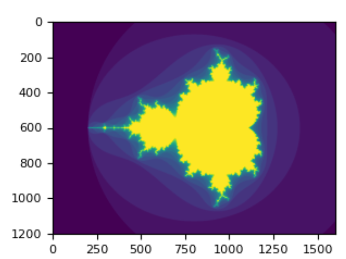
- You can look at the following example to see how to use boolean indexing to generate an image of the Mandelbrot set:
- Mandelbrot set:https://en.wikipedia.org/wiki/Mandelbrot_set ```python import numpy as np import matplotlib.pyplot as plt
def mandelbrot(h, w, maxit=20, r=2): “””Returns an image of the Mandelbrot fractal of size (h,w).””” x = np.linspace(-2.5, 1.5, 4 h + 1) y = np.linspace(-1.5, 1.5, 3 w + 1) A, B = np.meshgrid(x, y) C = A + B * 1j z = np.zeros_like(C) divtime = maxit + np.zeros(z.shape, dtype=int)
for i in range(maxit):
    z = z**2 + C
    diverge = abs(z) > r                    # who is diverging
    div_now = diverge & (divtime == maxit)  # who is diverging now
    divtime[div_now] = i                    # note when
    z[diverge] = r                          # avoid diverging too much

return divtime
plt.imshow(mandelbrot(400, 400))
- The second way of indexing with booleans is more similar to integer indexing; for each dimension of the array we give a 1D boolean array selecting the slices we want:
```python
a = np.arange(12).reshape(3, 4)
b1 = np.array([False, True, True]) # first dim selection
b2 = np.array([True, False, True, False]) # second dim selection
# selecting rows
print(a[b1, :])
"""
array([[ 4, 5, 6, 7],
[ 8, 9, 10, 11]])
"""
# same thing
print(a[b1])
"""
array([[ 4, 5, 6, 7],
[ 8, 9, 10, 11]])
"""
# selecting columns
print(a[:, b2])
"""
array([[ 0, 2],
[ 4, 6],
[ 8, 10]])
"""
# a weird thing to do
# jy: array([ 4, 10])
print(a[b1, b2])
Note that the length of the 1D boolean array must coincide with the length of the dimension (or axis) you want to slice. In the previous example,
b1has length 3 (the number of rows ina), andb2(of length 4) is suitable to index the 2nd axis (columns) ofa.3)The
ix_()functionThe
ix_function can be used to combine different vectors so as to obtain the result for each n-uplet. For example, if you want to compute all thea+b*cfor all the triplets taken from each of the vectorsa,bandc:ix_:https://numpy.org/doc/stable/reference/generated/numpy.ix.html#numpy.ix ```python a = np.array([2, 3, 4, 5]) b = np.array([8, 5, 4]) c = np.array([5, 4, 6, 8, 3]) ax, bx, cx = np.ix_(a, b, c) print(ax) “”” array([[[2]],[[3]],
[[4]],
[[5]]]) “””
print(bx) “”” array([[[8], [5], [4]]]) “””
jy: array([[[5, 4, 6, 8, 3]]])
print(cx)
jy: ((4, 1, 1), (1, 3, 1), (1, 1, 5))
ax.shape, bx.shape, cx.shape
result = ax + bx * cx orint(result) “”” array([[[42, 34, 50, 66, 26], [27, 22, 32, 42, 17], [22, 18, 26, 34, 14]],
   [[43, 35, 51, 67, 27],
    [28, 23, 33, 43, 18],
    [23, 19, 27, 35, 15]],

   [[44, 36, 52, 68, 28],
    [29, 24, 34, 44, 19],
    [24, 20, 28, 36, 16]],

   [[45, 37, 53, 69, 29],
    [30, 25, 35, 45, 20],
    [25, 21, 29, 37, 17]]])
“””
jy: 17
print(result[3, 2, 4])
jy: 17
print(a[3] + b[2] * c[4])
- You could also implement the reduce as follows:
```python
def ufunc_reduce(ufct, *vectors):
   vs = np.ix_(*vectors)
   r = ufct.identity
   for v in vs:
       r = ufct(r, v)
   return r

print(ufunc_reduce(np.add, a, b, c))
"""
array([[[15, 14, 16, 18, 13],
        [12, 11, 13, 15, 10],
        [11, 10, 12, 14,  9]],

       [[16, 15, 17, 19, 14],
        [13, 12, 14, 16, 11],
        [12, 11, 13, 15, 10]],

       [[17, 16, 18, 20, 15],
        [14, 13, 15, 17, 12],
        [13, 12, 14, 16, 11]],

       [[18, 17, 19, 21, 16],
        [15, 14, 16, 18, 13],
        [14, 13, 15, 17, 12]]])
"""
The advantage of this version of reduce compared to the normal
ufunc.reduceis that it makes use of the broadcasting rules in order to avoid creating an argument array the size of the output times the number of vectors.- broadcasting rules:https://numpy.org/doc/stable/user/quickstart.html#broadcasting-rules
4)Indexing with strings
- broadcasting rules:https://numpy.org/doc/stable/user/quickstart.html#broadcasting-rules
参考:https://numpy.org/doc/stable/user/basics.rec.html#structured-arrays
7、Tricks and Tips
Here we give a list of short and useful tips.
1)”Automatic” Reshaping
To change the dimensions of an array, you can omit one of the sizes which will then be deduced automatically:
a = np.arange(30)
# -1 means "whatever is needed"
b = a.reshape((2, -1, 3))
# jy: (2, 5, 3)
print(b.shape)
print(b)
"""
array([[[ 0,  1,  2],
      [ 3,  4,  5],
      [ 6,  7,  8],
      [ 9, 10, 11],
      [12, 13, 14]],

     [[15, 16, 17],
      [18, 19, 20],
      [21, 22, 23],
      [24, 25, 26],
      [27, 28, 29]]])
"""
2)Vector Stacking
How do we construct a 2D array from a list of equally-sized row vectors? In MATLAB this is quite easy: if
xandyare two vectors of the same length you only need dom=[x;y]. In NumPy this works via the functionscolumn_stack,dstack,hstackandvstack, depending on the dimension in which the stacking is to be done. For example: ```python x = np.arange(0, 10, 2) y = np.arange(5) m = np.vstack([x, y]) print(m) “”” array([[0, 2, 4, 6, 8],[0, 1, 2, 3, 4]])“””
xy = np.hstack([x, y])
jy: array([0, 2, 4, 6, 8, 0, 1, 2, 3, 4])
print(xy)
- The logic behind those functions in more than two dimensions can be strange.
- [https://numpy.org/doc/stable/user/numpy-for-matlab-users.html](https://numpy.org/doc/stable/user/numpy-for-matlab-users.html)
<a name="eF2JO"></a>
## 3)Histograms
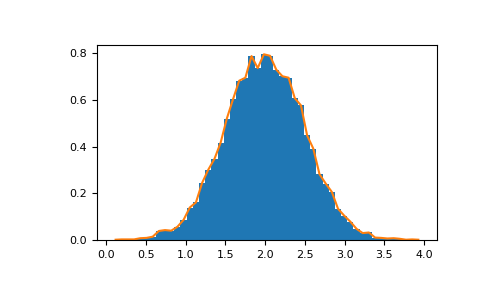
- The NumPy `histogram` function applied to an array returns a pair of vectors: the histogram of the array and a vector of the bin edges.
- Beware: `matplotlib` also has a function to build histograms (called `hist`, as in Matlab) that differs from the one in NumPy.
- The main difference is that `pylab.hist` plots the histogram automatically, while `numpy.histogram` only generates the data.
```python
import numpy as np
import matplotlib.pyplot as plt
rg = np.random.default_rng(1)
# Build a vector of 10000 normal deviates with variance 0.5^2 and mean 2
mu, sigma = 2, 0.5
v = rg.normal(mu, sigma, 10000)
# Plot a normalized histogram with 50 bins
# matplotlib version (plot)
plt.hist(v, bins=50, density=True)
# Compute the histogram with numpy and then plot it
# NumPy version (no plot)
(n, bins) = np.histogram(v, bins=50, density=True)
plt.plot(.5 * (bins[1:] + bins[:-1]), n)
- With Matplotlib >=3.4 you can also use
plt.stairs(n, bins).

若有收获,就点个赞吧
0 人点赞
