Unpaired image-to-image translation
The power of CycleGAN lies in being able to learn such transformations without one-to-one mapping between training data in source and target domains.
CycleGAN能够学习这种映射关系,而不需要源域和目标域之间的一一映射。
The need for a paired image in the target domain is eliminated by making a two-step transformation of source domain image - first by trying to map it to target domain and then back to the original image.
首先将图像映射到目标域,然后将其映射回源域,从而可以消除需要一一配对的问题。
Mapping the image to target domain is done using a generator network and the quality of this generated image is improved by pitching the generator against a discrimintor.
生成网络 — 实现图像到目标域之间的映射
鉴别器提高生成网络的图像质量
Adversarial Networks
We have a generator network and discriminator network playing against each other. The generator tries to produce samples from the desired distribution and the discriminator tries to predict if the sample is from the actual distribution or produced by the generator. The generator and discriminator are trained jointly. The effect this has is that eventually the generator learns to approximate the underlying distribution completely and the discriminator is left guessing randomly.
生成器尝试产生想要的分布,鉴别器尝试预测是真实分布还是生成器生成的分布。
生成器和鉴别器同时进行训练。
Cycle-Consistent
Adversarial training can, in theory, learn mappings G and F that produce outputs identically distributed as target domains Y and X respectively. However, with large enough capacity, a network can map the same set of input images to any random permutation of images in the target domain, where any of the learned mappings can induce an output distribution that matches the target distribution. Thus, an adversarial loss alone cannot guarantee that the learned function can map an individual input xi to a desired output yi.
To regularize the model, the authors introduce the constraint of cycle-consistency - if we transform from source distribution to target and then back again to source distribution, we should get samples from our source distribution.
为了使模型规范化,引入循环一致性约束。
有两个generator,一个是genA->B, 一个是genB->A
两个Discriminator, 一个是DiscA, 另一个是DiscB
Network Architecture
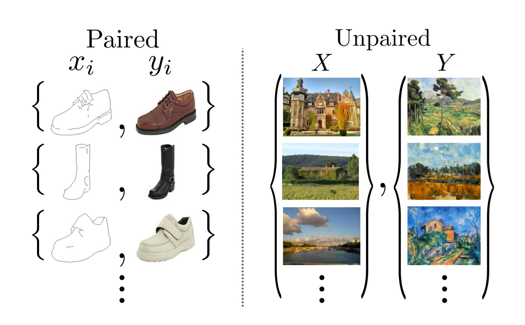
In a paired dataset, every image, say imgA, is manually mapped to some image, say imgB, in target domain, such that they share various features.
在一个成对的数据集中,每个图像都是手动映射到某个图像上的,使得它们在目标域上有不同的特征
Features that can be used to map an image (imgA/imgB)to its correspondingly mapped counterpart (imgB/imgA).
Basically, pairing is done to make input and output share some common features.
配对是为了让输入和输出有一些共性特征。
This mapping defines meaningful transformation of an image from one damain to another domain.
So, when we have paired dataset, generator must take an input, say inputA, from domain DA and map this image to an output image, say genB, which must be close to its mapped counterpart.
But we don’t have this luxury in unpaired dataset, there is no pre-defined meaningful transformation that we can learn, so, we will create it.
但在未配对的数据集中,我们没有这种奢侈,没有预先定义的有意义的转换可以学习,需要我们来创建
We need to make sure that there is some meaningful relation between input image and generated image.
我们需要确保输入图像和生成图像之间有一些有意义的关系
So, authors tried to enforce this by saying that Generator will map input image (inputA)from domain DA to some image in target domain DB , but to make sure that there is meaningful relation between these images, they must share some feature, features that can be used to map this output image back to input image, so there must be another generator that must be able to map back this output image back to original input. So, you can see this condition defining a meaningful mapping between inputA and genB.
映射的图像和输入图像必需共享一些特征,这些特征可以将输出图像映射回输入图像,所以必须有另一个生成器能够将输出图像映射回原始输入。
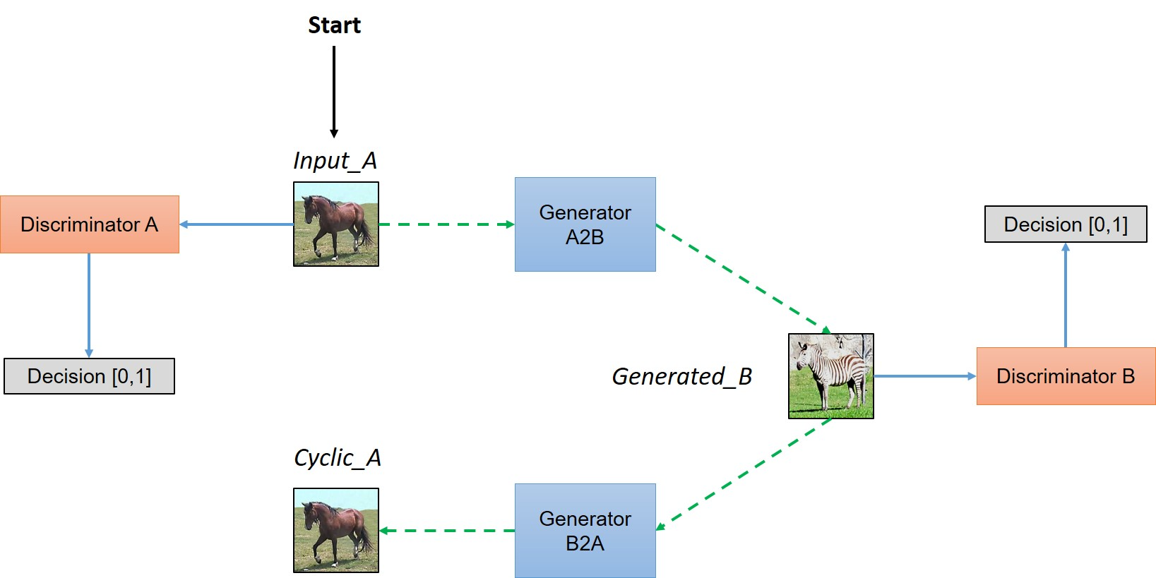
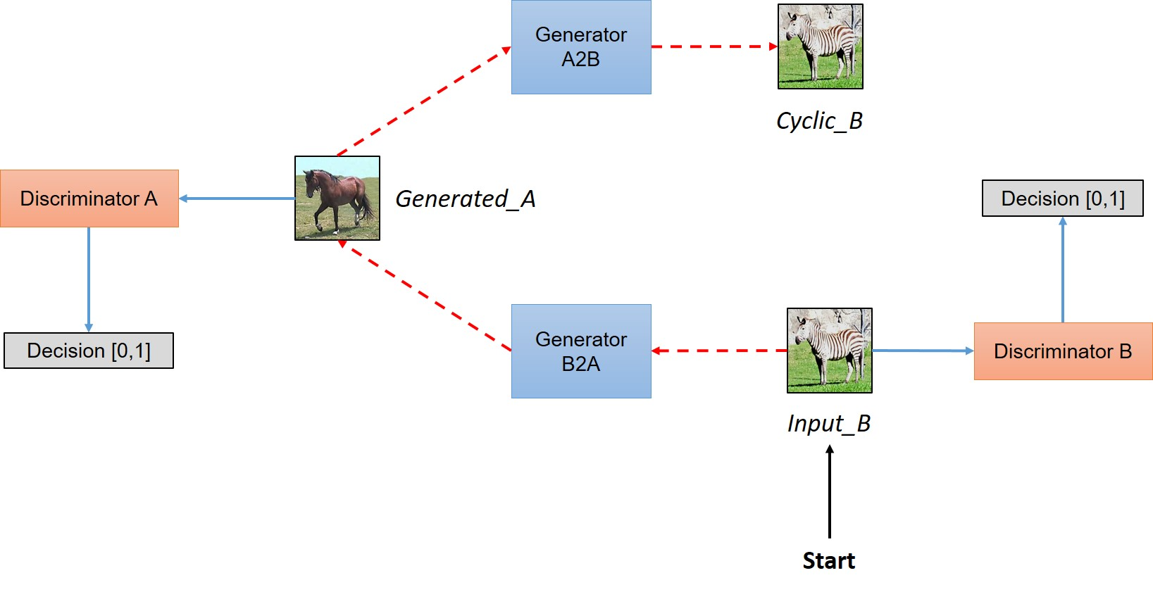
In a nutshell,the model works by taking an input image from domain DA which is fed to our first generator GeneratorA→B whose job is to transform a given image from domain DA to an image in target domain DB.
简而言之, 从域DA中提取一幅图像输入到我们的生成器GeneratorA→B中,该生成器的任务是将给定的图像从区域DA转化为区域DB中的图像。
新生成的图像然后被传送到另一个生成器Generator B→A中,转化为域DA中的图像,输出图像必须接近原始的输入图像
As you can see in above figure, two inputs are fed into each discriminator (one is original image corresponding to that domain and other is the generated image via a generator) and the job of discriminator is to distinguish between them, so that discriminator is able to defy the adversary (in this case generator) and reject images generated by it.
While the generator would like to make sure that these images get accepted by the discriminator, so it will try to generate images which are very close to original images in Class DB. (In fact, the generator and discriminator are actually playing a game whose Nash equilibrium is achieved when the generator’s distribution becomes same as the desired distribution)
Code
Building the generator
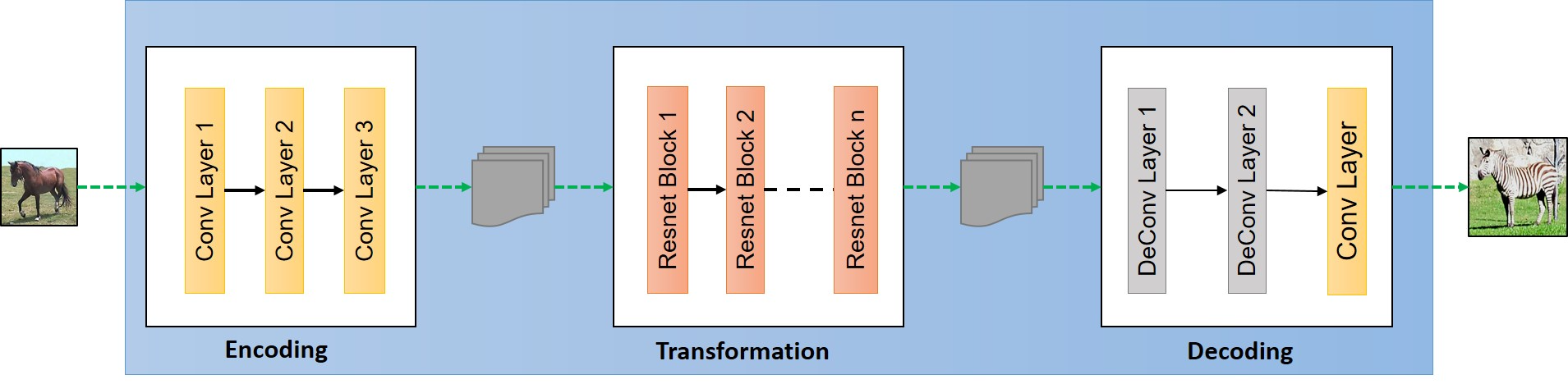
The generator have three components:
- Encoder
- Transformer
- Decoder
Following are the parameters we have used for the mode.
ngf = 32 # Number of filters in first layer of generatorndf = 64 # Number of filters in first layer of discriminatorbatch_size = 1 # batch_sizepool_size = 50 # pool_sizeimg_width = 256 # Imput image will of width 256img_height = 256 # Input image will be of height 256img_depth = 3 # RGB format
First three parameters are self explanatory and we will explain what pool_size means in the Generated Image Pool section.
Encoding:
For the purpose of simplicity, throughout the article we will assume that the input size is [256,256,3][256,256,3]. The first step is extracting the features from an image which is done a convolution network. To learn the basics about convolutional networks you can go through this very intuitive blog post by ujjwalkarn. As input a convolution network takes an image, size of filter window that we move over input image to extract out features and the stride size to decide how much we will move filter window after each step. So the first layer of encoding looks like this:
利用一个卷积神经网络来提取特征
编码器的第一层:
o_c1 = general_conv2d(input_gen,num_features=ngf,window_width=7,window_height=7,stride_width=1,stride_height=1)
input_gen is the input image to the generator,
num_features is the number of output features we extract out of the convolution layer, which can also be seen as number of different filters used to extract different features.
window_width and window_height denote the width and heigth of filter window that we will move accross the input image to extract features and similarly stride_width and stride_height defines the shift of filter patch after each step.
The output oc1 is a tensor of dimensions [256,256,64] which is again passed through another convolution layer. Here, ngf = 64 as mentioned earlier. I have defined the general_conv2d function. We can add other layers like relu or batch normalization layer but we are skipping the details of these layers in this tutorial.
def general_conv2d(inputconv, o_d=64, f_h=7, f_w=7, s_h=1, s_w=1):with tf.variable_scope(name):conv = tf.contrib.layers.conv2d(inputconv, num_features, [window_width, window_height], [stride_width, stride_height],padding, activation_fn=None, weights_initializer=tf.truncated_normal_initializer(stddev=stddev),biases_initializer=tf.constant_initializer(0.0))
Futher:
o_c2 = general_conv2d(o_c1, num_features=64*2, window_width=3, window_height=3, stride_width=2, stride_height=2)# o_c2.shape = (128, 128, 128)o_enc_A = general_conv2d(o_c2, num_features=64*4, window_width=3, window_height=3, stride_width=2, stride_height=2)# o_enc_A.shape = (64, 64, 256)
Each convolution layer leads to extraction of progressively higher level features. It can also be seen as compressing an image into 256 features vectors of size 64*64 each. We are now in good shape to transform this feature vector of a image in Domain DA to feature vector of an image in domain DB.
To summarize, we took an image from domain DADA of size [256,256,3] which we fed into our encoder to get output oAencoencA of size [64,64,256].
Transformation:
You can view these layers as combining different nearby features of an image and then based on these features making decision about how we would like to transform that feature vector/encoding of an image from DA to that of DB. So for this, authors have used 6 layer of resnet blocks as follow:
o_r1 = build_resnet_block(o_enc_A, num_features=64*4)o_r2 = build_resnet_block(o_r1, num_features=64*4)o_r3 = build_resnet_block(o_r2, num_features=64*4)o_r4 = build_resnet_block(o_r3, num_features=64*4)o_r5 = build_resnet_block(o_r4, num_features=64*4)o_enc_B = build_resnet_block(o_r5, num_features=64*4)
Here oBenc denotes the final output of this layer which will be of the size [64,64,256]. And as discussed ealier, this can be seens as the feature vector for an image in domain DB.
You must be wondering what is this build_resnet_block function and what does it do? build_resnet_block is a neural network layer which consists of two convolution layers where a residue of input is added to the output. This is done to ensure properties of input of previous layers are available for later layers as well, so that the their output do not deviate much from original input, otherwise the characteristics of original images will not be retained in the output and results will be very abrupt. As we discussed earlier, one of the primary aim fo the task is to retain the characteristic of original input like the size and shape of the object, so residual networks are a great fit for these kind of transformations. Resnet block can be summarized in following image
resnet block
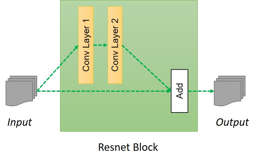
def resnet_blocks(input_res, num_features):out_res_1 = general_conv2d(input_res, num_features,window_width=3,window_heigth=3,stride_width=1,stride_heigth=1)out_res_2 = general_conv2d(out_res_1, num_features,window_width=3,window_heigth=3,stride_width=1,stride_heigth=1)return (out_res_2 + input_res)
Decoding
Up until now we have fed a feature vector oAenc into a transformation layer to get another feature vector oBenc of size [64,64,256].
Decoding step is exact opposite of Step 1, we will build back the low level features back from the feature vector. This is done by applying a deconvolution (or transpose convolution) layer.
o_d1 = general_deconv2d(o_enc_B, num_features=ngf*2 window_width=3, window_height=3, stride_width=2, stride_height=2)o_d2 = general_deconv2d(o_d1, num_features=ngf, window_width=3, window_height=3, stride_width=2, stride_height=2)
Finally we will convert this low level feature to image in domain DB as follow:
gen_B = general_conv2d(o_d2, num_features=3, window_width=7, window_height=7, stride_width=1, stride_height=1)
def build_generator(input_gen):o_c1 = general_conv2d(input_gen, num_features=ngf, window_width=7, window_height=7, stride_width=1, stride_height=1)o_c2 = general_conv2d(o_c1, num_features=ngf*2, window_width=3, window_height=3, stride_width=2, stride_height=2)o_enc_A = general_conv2d(o_c2, num_features=ngf*4, window_width=3, window_height=3, stride_width=2, stride_height=2)# Transformationo_r1 = build_resnet_block(o_enc_A, num_features=64*4)o_r2 = build_resnet_block(o_r1, num_features=64*4)o_r3 = build_resnet_block(o_r2, num_features=64*4)o_r4 = build_resnet_block(o_r3, num_features=64*4)o_r5 = build_resnet_block(o_r4, num_features=64*4)o_enc_B = build_resnet_block(o_r5, num_features=64*4)#Decodingo_d1 = general_deconv2d(o_enc_B, num_features=ngf*2 window_width=3, window_height=3, stride_width=2, stride_height=2)o_d2 = general_deconv2d(o_d1, num_features=ngf, window_width=3, window_height=3, stride_width=2, stride_height=2)gen_B = general_conv2d(o_d2, num_features=3, window_width=7, window_height=7, stride_width=1, stride_height=1)return gen_B
Build the discriminator
We discussed how to build a generator, however for adversarial training of the network we need to build a discriminator as well. The discriminator would take an image as an input and try to predict if it is an original or the output from the generator. Generator can be visualized in following image.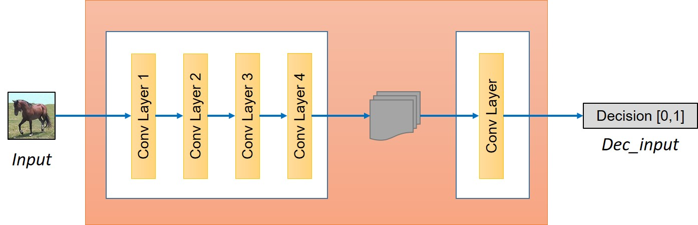
The discriminator is simply a convolution network in our case. First, we will extract the features from the image.
o_c1 = general_conv2d(input_disc, ndf, f, f, 2, 2)o_c2 = general_conv2d(o_c1, ndf*2, f, f, 2, 2)o_enc_A = general_conv2d(o_c2, ndf*4, f, f, 2, 2)o_c4 = general_conv2d(o_enc_A, ndf*8, f, f, 2, 2)
Next step is deciding whether these features belongs to that particular category or not. For that we will add a final convolution layer that produces a 1 dimensional output. Here, ndf denotes the number of features in initial layer of discriminator that one can vary or experiment with to get the best result.
decision = general_conv2d(o_c4, 1, f, f, 1, 1, 0.02)
We now have two main components of the model, namely Generator and Discriminator, and since we want to make this model work in both the direction i.e., from A→B and from B→A, we will have two Generators, namely GeneratorA→B and GeneratorB→A, and two Discriminators, namely DiscriminatorA and DiscriminatorB
Build the model
Before getting to loss funtion let us define the base and see how to take input, construct the model.
input_A = tf.placeholder(tf.float32, [batch_size, img_width, img_height, img_layer], name="input_A")input_B = tf.placeholder(tf.float32, [batch_size, img_width, img_height, img_layer], name="input_B")
These placeholders will act as input while defining our model as follow.
gen_B = build_generator(input_A, name="generator_AtoB")gen_A = build_generator(input_B, name="generator_BtoA")dec_A = build_discriminator(input_A, name="discriminator_A")dec_B = build_discriminator(input_B, name="discriminator_B")dec_gen_A = build_discriminator(gen_A, "discriminator_A")dec_gen_B = build_discriminator(gen_B, "discriminator_B")cyc_A = build_generator(gen_B, "generator_BtoA")cyc_B = build_generator(gen_A, "generator_AtoB")
Above variable names are quite intuitive in nature. gen represents image generated after using corresponding Generator and dec represents decision after feeding the corresponding input to the discriminator.
Loss function
By now we have two generators and two discriminators. We need to design the loss function in a way which accomplishes our goal. The loss function can be seen having four parts:
- Discriminator must approve all the original images of the corresponding categories.
- Discriminator must reject all the images which are generated by corresponding Generators to fool them.
- Generators must make the discriminators approve all the generated images, so as to fool them.
- The generated image must retain the property of original image, so if we generate a fake image using a generator say GeneratorA→B then we must be able to get back to original image using the another generator GeneratorB→A - it must satisfy cyclic-consistency.
Discriminator loss
鉴别器的损失
Part 1
Discriminator must be trained such that recommendation for images from category A must be as close to 1, and vice versa for discriminator B. So Discriminator A would like to minimize (DiscriminatorA(a)−1)2 and same goes for B as well. This can be implemented as:
鉴别器对来自类别A的图像的识别率必须接近于1
D_A_loss_1 = tf.reduce_mean(tf.squared_difference(dec_A,1))D_B_loss_1 = tf.reduce_mean(tf.squared_difference(dec_B,1))
识别生成器生成的图像为真的概率应该要接近于0
Part 2
Since, discriniator should be able to distinguish between generated and original images, it should also be predicting 0 for images produced by the generator, i.e. Discriminator A would like to minimize (DiscriminatorA(GeneratorB→A(b)))2. It can be calculated as follow:
鉴别器还要能识别生成的图像和原始图像
D_A_loss_2 = tf.reduce_mean(tf.square(dec_gen_A))D_B_loss_2 = tf.reduce_mean(tf.square(dec_gen_B))D_A_loss = (D_A_loss_1 + D_A_loss_2)/2D_B_loss = (D_B_loss_1 + D_B_loss_2)/2
Generator loss
Generator should eventually be able to fool the discriminator about the authencity of it’s generated images. This can done if the recommendation by discriminator for the generated images is as close to 1 as possible. So generator would like to minimize (DiscriminatorB(GeneratorA→B(a))−1)2
生成器应该最终能欺骗鉴别器
生成器对鉴别器产生图像的推荐值尽可能接近1
So the loss is:
g_loss_B_1 = tf.reduce_mean(tf.squared_difference(dec_gen_A,1))g_loss_A_1 = tf.reduce_mean(tf.squared_difference(dec_gen_A,1))
Cyclic loss
And the last one and one of the most important one is the cyclic loss that captures that we are able to get the image back using another generator and thus the difference between the original image and the cyclic image should be as small as possible.
原始图像和循环图像之间的差别应该尽可能小
cyc_loss = tf.reduce_mean(tf.abs(input_A-cyc_A)) + tf.reduce_mean(tf.abs(input_B-cyc_B))
The complete generator loss is then:
g_loss_A = g_loss_A_1 + 10*cyc_lossg_loss_B = g_loss_B_1 + 10*cyc_loss
The multiplicative factor of 10 for cyc_loss assigns more importance to cyclic loss than the discrimination loss.
Putting it together
With the loss function defined, all the is needed to train the model is to minimize the loss function w.r.t. model parameters.
d_A_trainer = optimizer.minimize(d_loss_A, var_list=d_A_vars)d_B_trainer = optimizer.minimize(d_loss_B, var_list=d_B_vars)g_A_trainer = optimizer.minimize(g_loss_A, var_list=g_A_vars)g_B_trainer = optimizer.minimize(g_loss_B, var_list=g_B_vars)
Reference

若有收获,就点个赞吧
0 人点赞
