Logistic回归
Logistic regression
This is a learning algorithm that you use when the output labels y in a supervised learning problem are all zero or one, so for binary classification problem.
If input x is a picture, you want an algorithm that can output a prediction which we’ll call y hat, which is your estimate of y.
x is an nx dimensional vector
given that the parameters of logistic regression will be w, which is also a nx dimensional vector, together with b which is just a real number
So given an input X and the parameters W and b, how can we generate the output y hat?
y^ = wTx + b
But this isn’t a very good algorithm for binary classification, because you want y hat to be the chance that Y is equal to one. So y hat should really be between zero and one.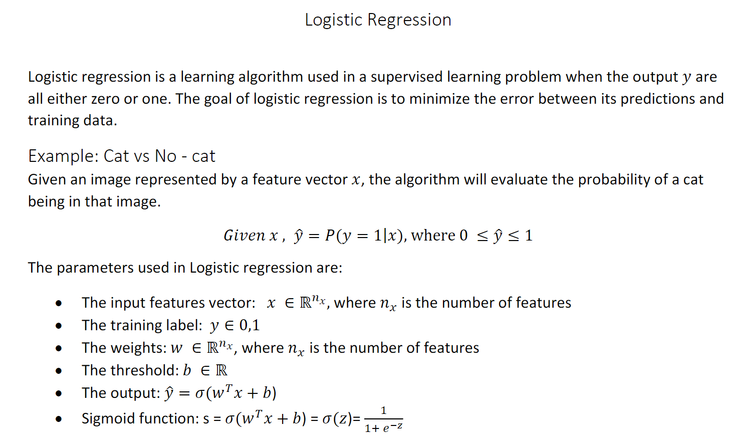
Sigmoid函数
wTx + b的值可能很大,也可能是负值,所以讲sigmoid函数作用到这个量上
y^ = sigmoid(wTx + b) 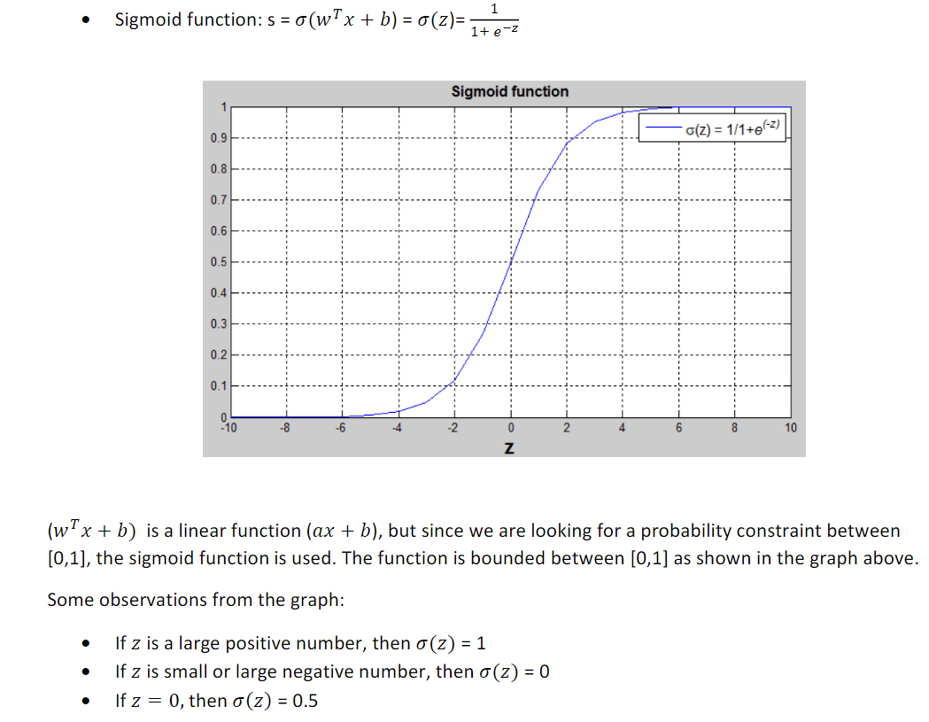
logistic回归损失函数
To train the parameter W and B of the logistic regression model, you need to define a cost function.
Your output y-hat is sigmoid of w transpose x plus b , where a sigmoid of Z is as defined here.
So to learn parameters for your model you’re given a training set of m training examples and it seems natural that you want to find parameters W and B, so that at least the outputs you have on the training set,
which we only write as y-hat that will be close to the ground truth labels y(i) that you got in the training set.
Your prediction on training sample(i) which is y-hat(i) is going to be obtained by taking the sigmoid function and applying it to w transpose x^(i) , the input that the training example plus B.
PS: the superscript parentheses i refers to data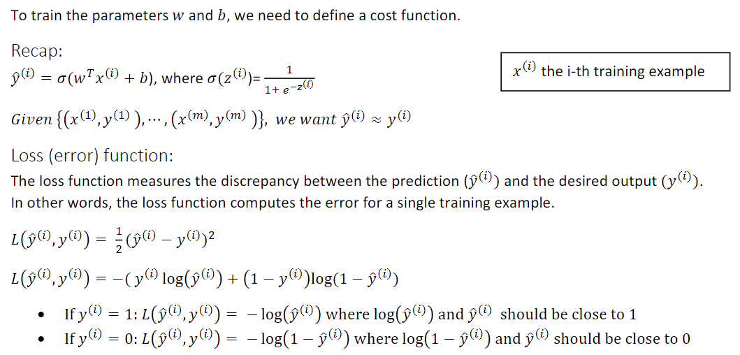
Loss function
We can use to measure how well our algorithm is doing.
when your algorithm outputs y-hat and the true label as Y to be the square error or one half a square error.
It turns out that you could do this, but in logistic regression people don’t usually do this. Because you find that the optimization problem which we talk about later becomes non-convex. So you end up with optimization problem with multiple local optima.
还有多个局部最优解
But the intuition to take away is that this function L called the loss function is a function you’ll need to define to measure how good our output y-hat is when the true lable is y.
As square error seems like it might be a reasonable choice, except that it makes gradient descent not work well.
So in logistic regression, we will actually define a different loss function that plays a similar role as square error, that will give us an optimization problem that is convex.
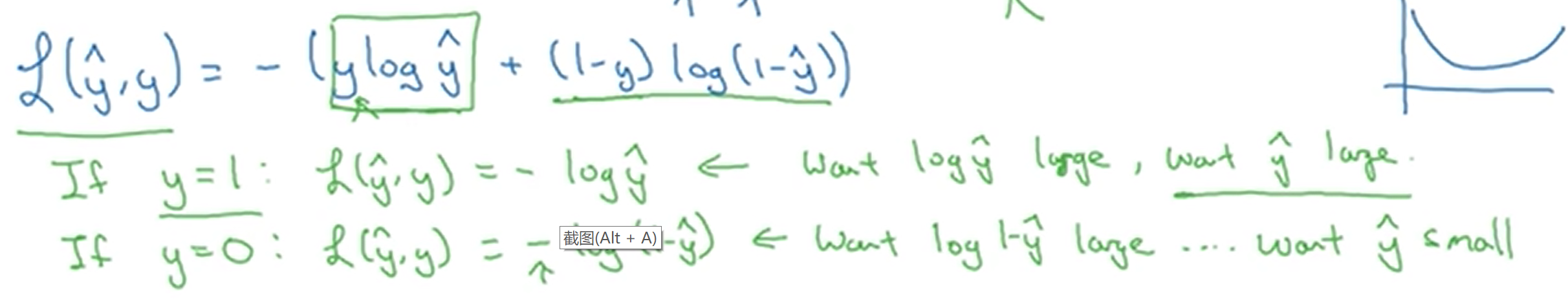
And again because y-hat has to be between zero and one. then your loss function will push the parameters to make y-hat as close to zero as possible
Finally, the loss function was defined with respect to a single training example.
It measure how well you’re doing on a single training example.
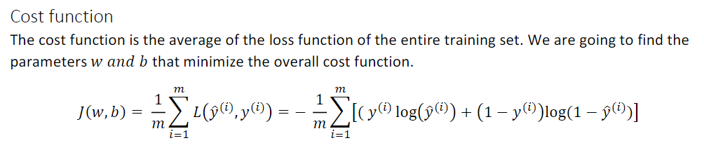
cost function
I’m now going to define something called the function, which measures how well you’re doing an entire training set.
And the cost function is the cost of your parameters.
梯度下降法
Loss function that measures how well you’re doing on the single training example.
You’ve also seen the cost function that measures how well your parameters w and b are doing on your entile training set.
Now let’s talk about how you can use the gradienet decent algorithm to train or to learn the parameters w and b on your training set.
logistic function and the cost function J
the cost function measures how well your parameters w and b are doing on the training set
So in order to learn the set of parameters w and b, it seems natural that we want to find w and b that make the cost function J(w,b) as small as possible.
The cost function J(w,b) is then some surface above these horizontal axes w and b.
So the height of the surface represents the value of J(w,b) at a certain point.
And what we want to do is really to find the value of w and b that corresponds to the minimum of the cost function J.
So to find a good value for the parameters what we’ll do is initialize w and b to some initial value maybe denoted by that little red dot.
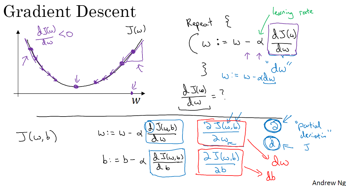
And what gradient descent does is it starts at that initial point and then takes a step in the steepest downhill direction. 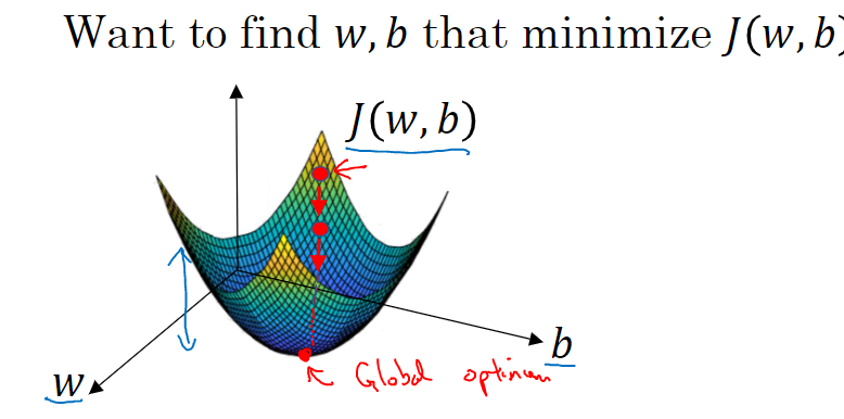
gradient descent does this we’re going to repeatedly carry out the following update
α —- the learning rate and controls how big a step we take on each iteration or gradient descent
derivative —- this basically the update or the change you want to make to the parameters w
计算图
probably say that the computations of a neural network are all organized of a forward path or a forward propagation step in which we compute the output of the neural network, followed by a backward pass or a back complication step which we use to compute gradients or compute derivatives.
The computation graph explains why it is organized this way
let’s say that we’re trying to compute a function J, which is a function of three variables a b and c
so the first thing we did was compute u equals B times C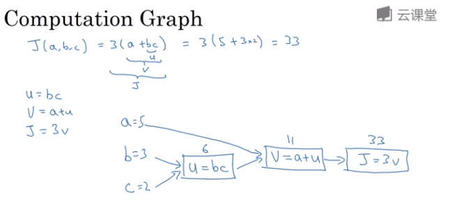
through a left-to-right pause you can compute the value of J
计算图的导数计算
how to use computation graph to figure out derivative calculations for that function J
chain rule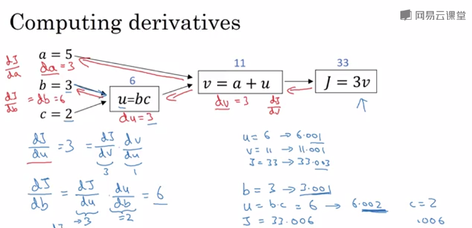
logistic回归中的梯度下降法
How to compute derivatives for you to implement gradient descent for logistic regression
where a is the output of the logistic regression and y is the ground truth label
and for this example let’s say we have only two features x1 and x2
so in order to compute z , we’ll need to input w1 w2 and b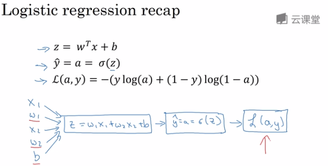
So in logistic regression what we want to do is to modify the parameters w and b, in order to reduce this loss
we’ve described before propagation steps of how you actually compute the loss on a single training example, now let’s talk about how you can go backwards to talk to compute the derivatives
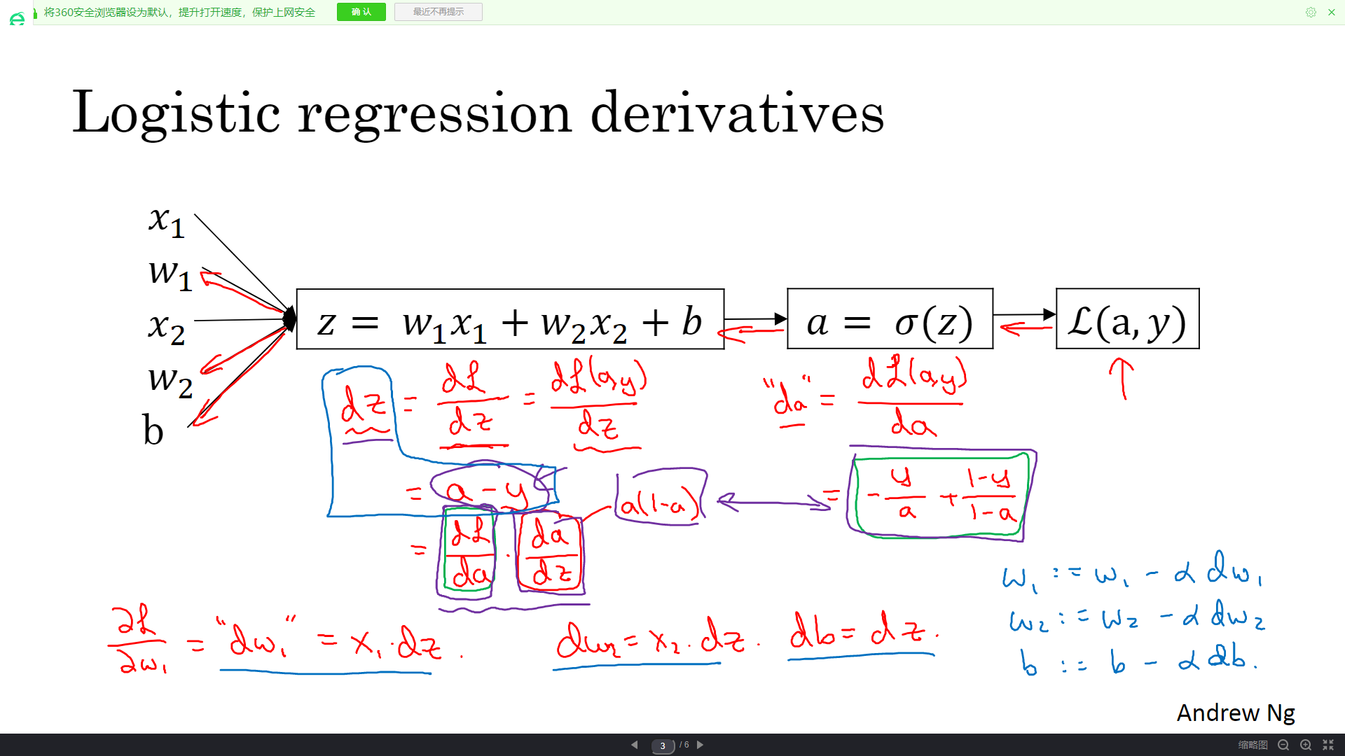
what we want to do is compute derivatives respect to this loss ,the first thing we want to do we’re going backwards is to compute the derivative of this loss with respect to this variable a
you can then go backwards and it turns out that you can show dz
this will be one step of gradient descent with respect to a single example
So you’ve seen how to compute derivatives and implement gradient descent for logistic regression with respect to a single training example
m个样本的梯度下降
now we want to do it for m training examples to get started
the definition of the cost function J(w,b) which you care about is this average right 1 over m sum from i equals 1 through m you konw the loss when your algorithm output a^i on the example y well you know a^i is the prediction on the I’ve trained example, which is sigmoid of z^i , which is equal to sigmoid of W transpose x^i plus b
so what we show in the previous slider is for any single training example how to compute the derivatives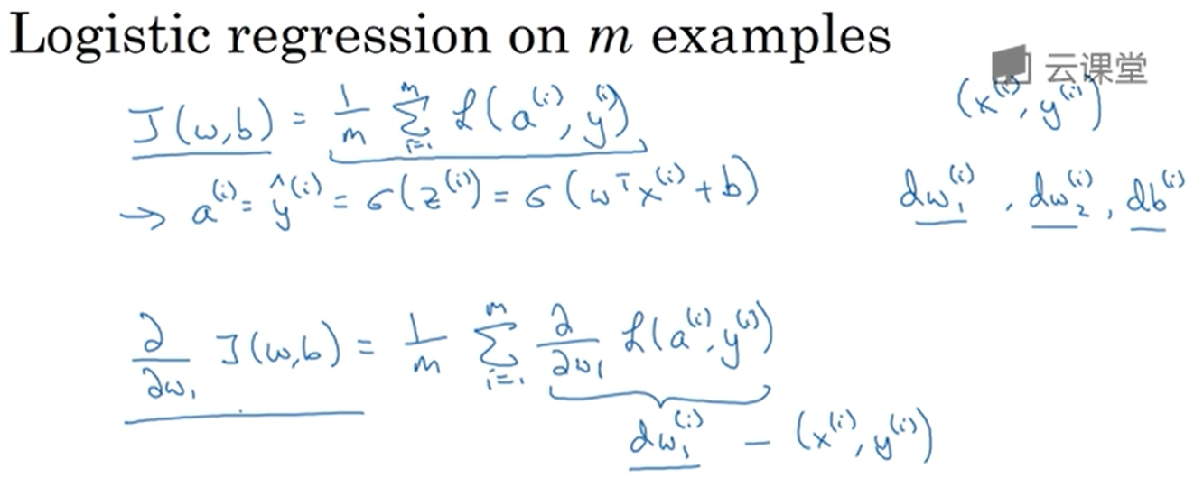
now you know the overall cost function with the sum was really the average of the 1 over m term of the individual losses
so it turns out that the derivative respect to say w1 of the overall cost function is also going to be the average of derivatives respect to w1 of the individual loss terms respect to w1 of the individual loss terms.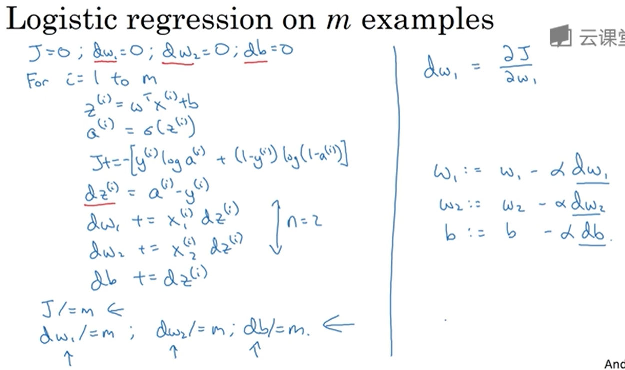

若有收获,就点个赞吧
0 人点赞
