GWAS 分析练习（二）关联分析

关联分析就是将突变与表型联系起来，如果表型是分类的，最简单的方法就是卡方检验。plink - -assoc 原理就是这样，但不能添加协变量，plink - -logistic可以做到这一点。如果表型是连续的数量表型，例如身高等，可以用 plink —linear ,也可以添加协助变量。
先将协变量信息写入到文件 SNP.covar，前两列是FID and IID，后面的列是协变量，主要有年龄、身高、体重等。表型文件 inhi.pheno1 前两列也是FID and IID，第三列是表型。

plink 关联分析

plink --bfile SNP --covar SNP.covar --logistic --hide-covar --out  bleeding 
plink --bfile SNP --covar SNP.covar --pheno inhi.pheno1 --linear --hide-covar --out  inhi1
plink --bfile SNP --covar SNP.covar --pheno inhi.pheno2 --logistic --hide-covar --out  inhi2

—covar designates the file to load covariates from. The file format is the same as for —pheno (optional header line, FID and IID in first two columns, covariates in remaining columns). By default, the main phenotype is set to missing if any covariate is missing; you can disable this with the ‘keep-pheno-on-missing-cov’ modifier.
—pheno causes phenotype values to be read from the 3rd column of the specified space- or tab-delimited file, instead of the .fam or .ped file. The first and second columns of that file must contain family and within-family IDs, respectively.

—covar 是添加协变量文件 —pheno 添加表型文件，同时会忽略原来 .fam 里的表型。
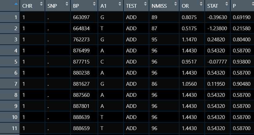
生成 .assoc.logistic 或者 .assoc.linear 文件，文件内容见下图。主要需要的数据就是P值，此值越小代表SNP与表型关系越显著。

做曼哈顿图（Manhattan）

参考作图的意义
https://www.jianshu.com/p/987859ae503c

使用R包作图

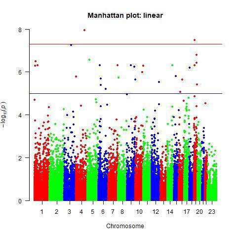
library(qqman)
bleeding <- read.table("../data/bleeding.assoc.logistic", head=TRUE)
bleeding <- bleeding[-which(is.na(bleeding[,9])),] 
##竟然有缺失值，导致报错，这个包竟然不能自动去除缺失值。上面步骤就是直接删除缺失的行。
jpeg("bleeding_manhattan.jpeg")
manhattan(bleeding,chr="CHR",bp="BP",p="P",snp="SNP", main = "Manhattan plot: logistic")
dev.off()

曼哈顿图其实就是散点图，横坐标代表染色体，纵坐标是P值对数，每个点就是一个SNP，点越高代表P值越小，和表型关系越显著。一般会高与5，6甚至达到8。

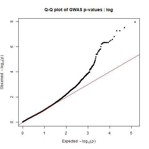
Q-Q plot ，P值越小的地方偏离直线越多，区别于预设的模型（随机分布），才证明我们挑出的关联的SNP越可靠。同样参考https://www.jianshu.com/p/987859ae503c

进一步分析

可以将显著相关的SNP进行注释