- 1. Explain a linear function with no interactions
- 2. Explain a linear model with one interaction
- simulate some binary data and a linear outcome with an interaction term
- note we make the features in X perfectly independent of each other to make
- it easy to solve for the exact SHAP values
- train a model with single tree
- make sure the SHAP values add up to marginal predictions
This notebook shows how the SHAP interaction values for a very simple function are computed. We start with a simple linear function, and then add an interaction term to see how it changes the SHAP values and the SHAP interaction values.
import xgboost as xgbimport numpy as npimport shap
1. Explain a linear function with no interactions
# simulate some binary data and a linear outcome with an interaction term# note we make the features in X perfectly independent of each other to make# it easy to solve for the exact SHAP valuesN = 2000X = np.zeros((N, 5))X[:1000, 0] = 1X[:500, 1] = 1X[1000:1500, 1] = 1X[:250, 2] = 1X[500:750, 2] = 1X[1000:1250, 2] = 1X[1500:1750, 2] = 1X[:, 0:3] -= 0.5y = 2 * X[:,0] - 3 * X[:, 1]# ensure the variables are independentnp.cov(X.T)# and mean centeredX.mean(0)
np.cov 函数用来计算协方差矩阵,如果输入只有一个数组的话,那就是计算方差
# train a model with single treeXd = xgb.DMatrix(X, label=y)model = xgb.train({'eta': 1,'max_depth': 3,'base_score': 0,'lambda': 0}, Xd, 1)print("Model error =", np.linalg.norm(y - model.predict(Xd)))print(model.get_dump(with_stats=True)[0])# Model error = 0.0# 0:[f1<0] yes=1,no=2,missing=1,gain=4500,cover=2000# 1:[f0<0] yes=3,no=4,missing=3,gain=1000,cover=1000# 3:leaf=0.5,cover=500# 4:leaf=2.5,cover=500# 2:[f0<0] yes=5,no=6,missing=5,gain=1000,cover=1000# 5:leaf=-2.5,cover=500# 6:leaf=-0.5,cover=500
:::info 解释一下上面代码: ::: :::success
- XGB 参数中
base_score表示对于所有样本预测为正样本的全局偏置,如果迭代次数够多,改变这个参数对结果不会有影响。将 base_score 设置为#(正样本)/#(所有样本)可减少迭代次数 np.linalg.norm表示对输入数组求范式,默认为,公式:
model.get_dump表示查看基分类器的决策树如何选择特征来进行分裂的,with_stats设置为True表示输出分裂统计信息 :::
# make sure the SHAP values add up to marginal predictionspred = model.predict(Xd, output_margin=True)explainer = shap.TreeExplainer(model)shap_values = explainer.shap_values(Xd)np.abs(shap_values.sum(1) + explainer.expected_value - pred).max() # 0
:::info
解释一下上面的代码:
:::
:::success
model.predict方法中output_margin参数,设置为True时,输出的不是概率值而是每个样本在 XGB 生成的所有树中叶子节点的累加值explainer.expected_value为样本期望值 :::
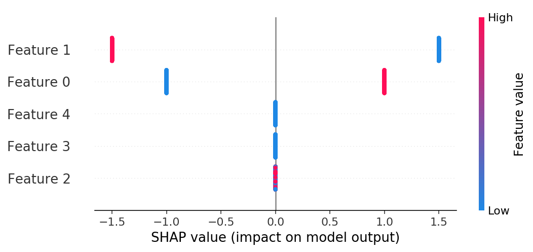
If we build a summary plot we see that only features 1 and 2 have any effect, and that their effects only have two possible magnitudes (one for -0.5 and for 0.5).
shap.summary_plot(shap_values, X)

# train a linear modelfrom sklearn import linear_modellr = linear_model.LinearRegression()lr.fit(X, y)lr_pred = lr.predict(X)lr.coef_.round(2) # array([ 2., -3., 0., 0., 0.])# Make sure the computed SHAP values match the true SHAP values# (we can compute the true SHAP values directly for this simple case)main_effect_shap_values = lr.coef_ * (X - X.mean(0))np.linalg.norm(shap_values - main_effect_shap_values) # 1.654243349044798e-13
1.1 SHAP Interaction Values
Note that when there are no interactions present the SHAP interaction values are just a diagonal matrix with the SHAP values on the diagonal(对角线).
shap_interaction_values = explainer.shap_interaction_values(Xd)shap_interaction_values[0]# array([[ 1. , 0. , 0. , 0. , 0. ],# [ 0. , -1.5, 0. , 0. , 0. ],# [ 0. , 0. , 0. , 0. , 0. ],# [ 0. , 0. , 0. , 0. , 0. ],# [ 0. , 0. , 0. , 0. , 0. ]], dtype=float32)# ensure the SHAP interaction values sum to the marginal predictionsnp.abs(shap_interaction_values.sum((1, 2)) + explainer.expected_value - pred).max() # 0# ensure the main effects from the SHAP interaction values match those from a linear modeldinds = np.diag_indices(shap_interaction_values.shape[1])total = 0for i in range(N):for j in range(5):total += np.abs(shap_interaction_values[i, j, j] - main_effect_shap_values[i, j])total # 1.0533118387982904e-11
:::info 解释: ::: :::success
np.diag_indices返回一组索引,用来访问 N x N 数组的对角线 :::2. Explain a linear model with one interaction
```pythonsimulate some binary data and a linear outcome with an interaction term
note we make the features in X perfectly independent of each other to make
it easy to solve for the exact SHAP values
N = 2000 X = np.zeros((N, 5)) X[:1000, 0] = 1
X[:500, 1] = 1 X[1000:1500, 1] = 1
X[:250, 2] = 1 X[500:750, 2] = 1 X[1000:1250, 2] = 1 X[1500:1750, 2] = 1
X[:125, 3] = 1 X[250:375, 3] = 1 X[500:625, 3] = 1 X[750:875, 3] = 1 X[1000:1125, 3] = 1 X[1250:1375, 3] = 1 X[1500:1625, 3] = 1 X[1750:1875, 3] = 1 X[:,:4] -= 0.4999 # we can’t exactly mean center the data or XGBoost has trouble finding the splits y = 2 X[:, 0] - 3 X[:, 1] + 2 X[:, 1] X[:, 2]
X.mean(0) # array([1.e-04, 1.e-04, 1.e-04, 1.e-04, 0.e+00])
train a model with single tree
Xd = xgb.DMatrix(X, label=y) model = xgb.train({‘eta’: 1, ‘max_depth’: 4, ‘base_score’: 0, “lambda”: 0}, Xd, 1) print(“Model error =”, np.linalg.norm(y-model.predict(Xd))) print(model.get_dump(with_stats=True)[0])
make sure the SHAP values add up to marginal predictions
pred = model.predict(Xd, output_margin=True) explainer = shap.TreeExplainer(model) shap_values = explainer.shap_values(Xd) np.abs(shap_values.sum(1) + explainer.expected_value - pred).max() # 4.7683716e-07
输出结果:
Model error = 1.7365037830677591e-06 0:[f1<0.000100001693] yes=1,no=2,missing=1,gain=4499.40039,cover=2000 1:[f0<0.000100001693] yes=3,no=4,missing=3,gain=999.999756,cover=1000 3:[f2<0.000100001693] yes=7,no=8,missing=7,gain=124.949997,cover=500 7:leaf=0.99970001,cover=250 8:leaf=-9.99800031e-05,cover=250 4:[f2<0.000100001693] yes=9,no=10,missing=9,gain=124.949951,cover=500 9:leaf=2.99970007,cover=250 10:leaf=1.99989998,cover=250 2:[f0<0.000100001693] yes=5,no=6,missing=5,gain=999.999756,cover=1000 5:[f2<0.000100001693] yes=11,no=12,missing=11,gain=125.050049,cover=500 11:leaf=-3.0000999,cover=250 12:leaf=-1.99989998,cover=250 6:[f2<0.000100001693] yes=13,no=14,missing=13,gain=125.050018,cover=500 13:leaf=-1.00010002,cover=250 14:leaf=0.000100019999,cover=250
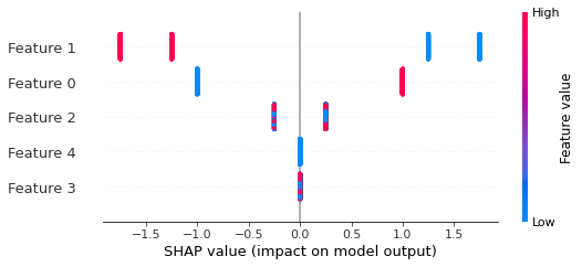
If we build a summary plot we see that now only features 3 and 4 don't matter, and that feature 1 can have four possible effect sizes due to interactions.```pythonshap.summary_plot(shap_values, X)

# train a linear modellr = linear_model.LinearRegression()lr.fit(X, y)lr_pred = lr.predict(X)lr.coef_.round(2) # array([ 2., -3., 0., 0., 0.])# Note that the SHAP values no longer match the main effects because they now include interaction effectsmain_effect_shap_values = lr.coef_ * (X - X.mean(0))np.linalg.norm(shap_values - main_effect_shap_values) # 15.811389093449788
2.1 SHAP interaction values
# SHAP interaction contributions:shap_interaction_values = explainer.shap_interaction_values(Xd)shap_interaction_values[0].round(2)# Output:# array([[ 1. , 0. , 0. , 0. , 0. ],# [ 0. , -1.5 , 0.25, 0. , 0. ],# [ 0. , 0.25, 0. , 0. , 0. ],# [ 0. , 0. , 0. , 0. , 0. ],# [ 0. , 0. , 0. , 0. , 0. ]], dtype=float32)# ensure the SHAP interaction values sum to the marginal predictionsnp.abs(shap_interaction_values.sum((1, 2)) + explainer.expected_value - pred).max()# Output: 4.7683716e-07# ensure the main effects from the SHAP interaction values match those from a linear model.# while the main effects no longer match the SHAP values when interactions are present, they do match# the main effects on the diagonal of the SHAP interaction value matrixdinds = np.diag_indices(shap_interaction_values.shape[1])total = 0for i in range(N):for j in range(5):total += np.abs(shap_interaction_values[i, j, j] - main_effect_shap_values[i, j])total # 0.4000067711135082
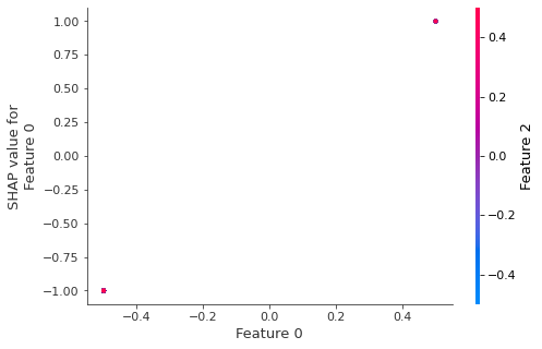
If we build a dependence plot for feature 0 we that it only takes two values and that these values are entirely dependent on the value of the feature (the value of feature 0 entirely determines it’s effect because it has no interactions with other features).
shap.dependence_plot(0, shap_values, X)

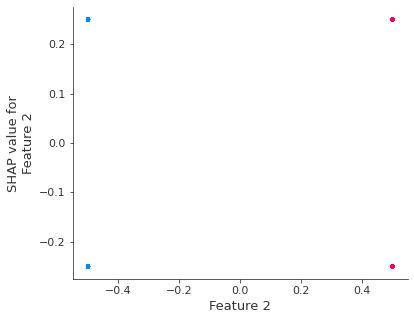
In contrast if we build a dependence plot for feature 2 we see that it takes 4 possible values and they are not entirely determined by the value of feature 2, instead they also depend on the value of feature 3. This vertical spread in a dependence plot represents the effects of non-linear interactions.
shap.dependence_plot(2, shap_values, X)


