- 1、Statistical learning: the setting and the estimator object in scikit-learn
- 2、Supervised learning: predicting an output variable from high-dimensional observations
- 3、Model selection: choosing estimators and their parameters
- 4、Unsupervised learning: seeking representations of the data
- these were introduced in skimage-0.14
- #
- Generate data
- Resize it to 20% of the original size to speed up the processing
- Applying a Gaussian filter for smoothing prior to down-scaling
- reduces aliasing artifacts.
- #
- Define the structure A of the data. Pixels connected to their neighbors.
- #
- Compute clustering
- #
- Plot the results on an image
- 5、Decompositions: from a signal to components and loadings
- 6、Putting it all together
🚀 原文链接:https://scikit-learn.org/stable/tutorial/statistical_inference/index.html
1、Statistical learning: the setting and the estimator object in scikit-learn
📄 原文链接:https://scikit-learn.org/stable/tutorial/statistical_inference/settings.html
1.1 Datasets
Scikit-learn deals with learning information from one or more datasets that are represented as 2D arrays. They can be understood as a list of multi-dimensional observations. We say that the first axis of these arrays is the samples axis, while the second is the features axis.
**
A simple example shipped with scikit-learn: iris dataset
It is made of 150 observations of irises(iris复数), each described by 4 features: their sepal(萼片) and petal(花瓣) length and width, as detailed in iris.DESCR.
>>> from sklearn import datasets>>> iris = datasets.load_iris()>>> data = iris.data>>> data.shape(150, 4)
When the data is not initially in the (n_samples, n_features) shape, it needs to be preprocessed in order to be used by scikit-learn.
An example of reshaping data would be the digits dataset The digits dataset is made of 1797 8x8 images of hand-written digits
>>> digits = datasets.load_digits()>>> digits.images.shape(1797, 8, 8)>>> import matplotlib.pyplot as plt>>> plt.imshow(digits.images[-1], cmap=plt.cm.gray_r)<matplotlib.image.AxesImage object at ...>
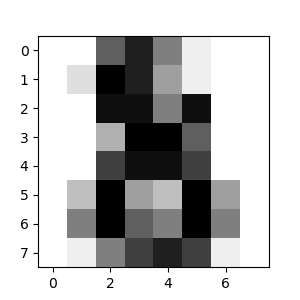
To use this dataset with scikit-learn, we transform each 8x8 image into a feature vector of length 64
>>> data = digits.images.reshape((digits.images.shape[0], -1))
1.2 Estimators objects
Fitting data: the main API implemented by scikit-learn is that of the estimator. An estimator is any object that learns from data; it may be a classification, regression or clustering algorithm or a transformer that extracts/filters useful features from raw data.
All estimator objects expose(暴露) a fit method that takes a dataset (usually a 2-d array):
>>> estimator.fit(data)
Estimator parameters: All the parameters of an estimator can be set when it is instantiated(实例化) or by modifying the corresponding attribute:
>>> estimator = Estimator(param1=1, param2=2)>>> estimator.param11
Estimated parameters: When data is fitted with an estimator, parameters are estimated from the data at hand. All the estimated parameters are attributes of the estimator object ending by an underscore(下划线):
>>> estimator.estimated_param_
2、Supervised learning: predicting an output variable from high-dimensional observations
📄 原文链接:https://scikit-learn.org/stable/tutorial/statistical_inference/supervised_learning.html
:::info
The problem solved in supervised learning
Supervised learning consists in learning the link between two datasets: the observed data X and an external variable y that we are trying to predict, usually called “target” or “labels”. Most often, y is a 1D array of length n_samples.
All supervised estimators in scikit-learn implement a fit(X, y) method to fit the model and a predict(X) method that, given unlabeled observations X, returns the predicted labels y.:::
:::info
Vocabulary: classification and regression
If the prediction task is to classify the observations in a set of finite(限定的) labels, in other words to “name” the objects observed, the task is said to be a classification task. On the other hand, if the goal is to predict a continuous target variable, it is said to be a regression task.
When doing classification in scikit-learn, y is a vector of integers or strings. Note: See the Introduction to machine learning with scikit-learn Tutorial for a quick run-through on the basic machine learning vocabulary used within scikit-learn.:::
2.1 Nearest neighbor and the curse of dimensionality
Classifying irises:
The iris dataset is a classification task consisting in identifying 3 different types of irises (Setosa, Versicolour, and Virginica) from their petal and sepal length and width:
>>> import numpy as np>>> from sklearn import datasets>>> iris_X, iris_y = datasets.load_iris(return_X_y=True)>>> np.unique(iris_y)array([0, 1, 2])
1) k-Nearest neighbors classifier
The simplest possible classifier is the nearest neighbor: given a new observation X_test, find in the training set (i.e. the data used to train the estimator) the observation with the closest feature vector. (Please see the Nearest Neighbors section of the online Scikit-learn documentation for more information about this type of classifier.)
Training set and testing set While experimenting with any learning algorithm, it is important not to test the prediction of an estimator on the data used to fit the estimator as this would not be evaluating the performance of the estimator on new data. This is why datasets are often split into train and test data.
KNN (k nearest neighbors) classification example: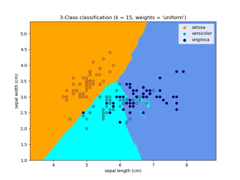
# Split iris data in train and test data# A random permutation, to split the data randomlyimport numpy as npfrom sklearn.neighbors import KNeighborsClassifiernp.random.seed(0)indices = np.random.permutation(len(iris_X))iris_X_train = iris_X[indices[:-10]]iris_y_train = iris_y[indices[:-10]]iris_X_test = iris_X[indices[-10:]]iris_y_test = iris_y[indices[-10:]]# Create and fit a nearest-neighbor classifierknn = KNeighborsClassifier()knn.fit(iris_X_train, iris_y_train)knn.predict(iris_X_test) # array([1, 2, 1, 0, 0, 0, 2, 1, 2, 0])iris_y_test # array([1, 1, 1, 0, 0, 0, 2, 1, 2, 0])
2) The curse(灾难) of dimensionality
For an estimator to be effective, you need the distance between neighboring points to be less than some value  , which depends on the problem. In one dimension, this requires on average
  points. In the context of the above
  -NN example, if the data is described by just one feature with values ranging from 0 to 1 and with
  training observations, then new data will be no further away than
  . Therefore, the nearest neighbor decision rule will be efficient as soon as is small compared to the scale of between-class feature variations(变化).
If the number of features is  , you now require
  points. Let’s say that we require 10 points in one dimension: now
  points are required in dimensions to pave(铺垫) the [0,1] space. As becomes large, the number of training points required for a good estimator grows exponentially(以指数方式).
For example, if each point is just a single number (8 bytes), then an effective -NN estimator in a paltry(微不足道的)  dimensions would require more training data than the current estimated size of the entire internet (±1000 Exabytes or so).
This is called the curse of dimensionality and is a core problem that machine learning addresses.
2.2 Linear model: from regression to sparsity
:::info
Diabetes dataset
The diabetes(糖尿病) dataset consists of 10 physiological(生理学的) variables (age, sex, weight, blood pressure) measure on 442 patients, and an indication of disease(病) progression after one year:
:::
>>> diabetes_X, diabetes_y = datasets.load_diabetes(return_X_y=True)>>> diabetes_X_train = diabetes_X[:-20]>>> diabetes_X_test = diabetes_X[-20:]>>> diabetes_y_train = diabetes_y[:-20]>>> diabetes_y_test = diabetes_y[-20:]
The task at hand is to predict disease progression from physiological variables.
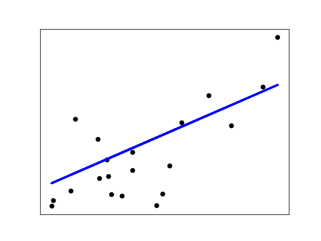
1) Linear regression
LinearRegression, in its simplest form, fits a linear model to the data set by adjusting a set of parameters in order to make the sum of the squared residuals(残差) of the model as small as possible.
Linear models: 
 : data
 : target variable
 : Coefficients
 : Observation noise
>>> from sklearn import linear_model>>> regr = linear_model.LinearRegression()>>> regr.fit(diabetes_X_train, diabetes_y_train)LinearRegression()>>> print(regr.coef_)[ 0.30349955 -237.63931533 510.53060544 327.73698041 -814.13170937492.81458798 102.84845219 184.60648906 743.51961675 76.09517222]# The mean square error>>> np.mean((regr.predict(diabetes_X_test) - diabetes_y_test) ** 2)2004.56760268...# Explained variance score: 1 is perfect prediction# and 0 means that there is no linear relationship# between X and y.>>> regr.score(diabetes_X_test, diabetes_y_test)0.5850753022690...
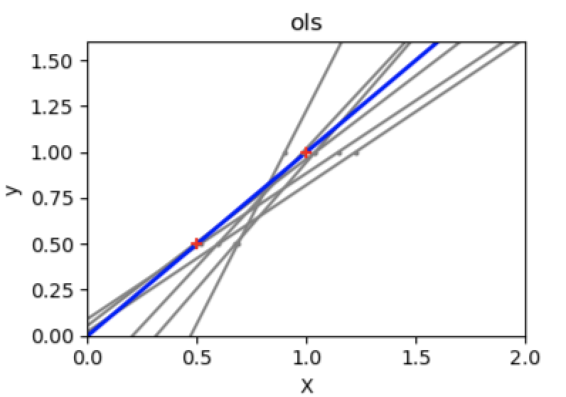
2) Shrinkage
If there are few data points per dimension, noise in the observations induces high variance:
import matplotlib.pyplot as pltX = np.c_[ .5, 1].Ty = [.5, 1]test = np.c_[ 0, 2].Tregr = linear_model.LinearRegression()plt.figure()np.random.seed(0)for _ in range(6):this_X = .1 * np.random.normal(size=(2, 1)) + Xregr.fit(this_X, y)plt.plot(test, regr.predict(test))plt.scatter(this_X, y, s=3)
A solution in high-dimensional statistical learning is to shrink(缩小) the regression coefficients to zero: any two randomly chosen set of observations are likely to be uncorrelated. This is called Ridge regression:
regr = linear_model.Ridge(alpha=.1)plt.figure()np.random.seed(0)for _ in range(6):this_X = .1 * np.random.normal(size=(2, 1)) + Xregr.fit(this_X, y)plt.plot(test, regr.predict(test))plt.scatter(this_X, y, s=3)
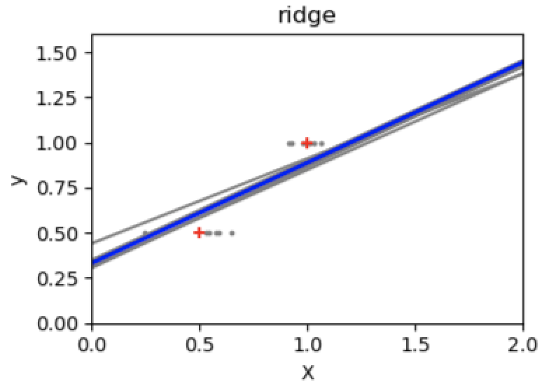
This is an example of bias/variance **tradeoff(权衡)**: the larger the ridge alpha parameter, the higher the bias and the lower the variance.
We can choose alpha to minimize left out error, this time using the diabetes dataset rather than our synthetic data:
alphas = np.logspace(-4, -1, 6)print([regr.set_params(alpha=alpha).fit(diabetes_X_train, diabetes_y_train).score(diabetes_X_test, diabetes_y_test)for alpha in alphas])# [0.5851110683883..., 0.5852073015444..., 0.5854677540698...,# 0.5855512036503..., 0.5830717085554..., 0.57058999437...]
Note: Capturing in the fitted parameters noise that prevents the model to generalize to new data is called > overfitting. The bias introduced by the ridge regression is called a > regularization.
3) Sparsity
Note:
A representation of the full diabetes dataset would involve 11 dimensions (10 feature dimensions and one of the target variable). It is hard to develop an intuition(直觉) on such representation, but it may be useful to keep in mind that it would be a fairly(公平地) empty space.
We can see that, although feature 2 has a strong coefficient on the full model, it conveys little information on y when considered with feature 1.
To improve the conditioning of the problem (i.e. mitigating(缓和) the The curse of dimensionality), it would be interesting to select only the informative features and set non-informative ones, like feature 2 to 0. Ridge regression will decrease their contribution, but not set them to zero. Another penalization(惩罚) approach, called Lasso (least absolute shrinkage(最小绝对收缩率) and selection operator), can set some coefficients to zero. Such methods are called sparse method and sparsity(稀疏) can be seen as an application of Occam’s razor: prefer simpler models.
regr = linear_model.Lasso()scores = [regr.set_params(alpha=alpha).fit(diabetes_X_train, diabetes_y_train).score(diabetes_X_test, diabetes_y_test)for alpha in alphas]>>> best_alpha = alphas[scores.index(max(scores))]>>> regr.alpha = best_alpha>>> regr.fit(diabetes_X_train, diabetes_y_train)Lasso(alpha=0.025118864315095794)>>> print(regr.coef_)[ 0. -212.437... 517.194... 313.779... -160.830...-0. -187.195... 69.382... 508.660... 71.842...]
:::info
Different algorithms for the same problem
Different algorithms can be used to solve the same mathematical problem. For instance the Lasso object in scikit-learn solves the lasso regression problem using a coordinate descent method, that is efficient on large datasets. However, scikit-learn also provides the LassoLars object using the LARS algorithm, which is very efficient for problems in which the weight vector estimated is very sparse (i.e. problems with very few observations).
:::
4) Classification
For classification, as in the labeling iris task, linear regression is not the right approach as it will give too much weight to data far from the decision frontier(绝对边界). A linear approach is to fit a sigmoid function or logistic function: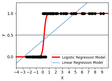

>>> log = linear_model.LogisticRegression(C=1e5)>>> log.fit(iris_X_train, iris_y_train)LogisticRegression(C=100000.0)
This is known as LogisticRegression.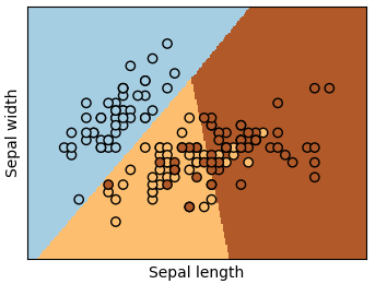 :::info
Multiclass classification
:::info
Multiclass classification
If you have several classes to predict, an option often used is to fit one-versus-all classifiers and then use a voting heuristic(启发) for the final decision.
:::
:::info
Shrinkage and sparsity with logistic regression
The C parameter controls the amount of regularization in the LogisticRegression object: a large value for C results in less regularization. penalty="l2" gives Shrinkage (i.e. non-sparse coefficients), while penalty="l1" gives Sparsity.
:::
:::info
Exercise
Try classifying the digits dataset with nearest neighbors and a linear model. Leave out the last 10% and test prediction performance on these observations. A solution can be downloaded here.
:::
from sklearn import datasets, neighbors, linear_modelX_digits, y_digits = datasets.load_digits(return_X_y=True)X_digits = X_digits / X_digits.max()
2.3 Support vector machines (SVMs)
1) Linear SVMs
Support Vector Machines belong to the discriminant(判别式的) model family: they try to find a combination of samples to build a plane(平面) maximizing the margin between the two classes. Regularization is set by the C parameter: a small value for C means the margin is calculated using many or all of the observations around the separating line (more regularization); a large value for C means the margin is calculated on observations close to the separating line (less regularization).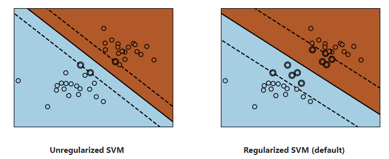
:::info Example:
SVMs can be used in regression –SVR (Support Vector Regression)–, or in classification –SVC (Support Vector Classification).
>>> from sklearn import svm>>> svc = svm.SVC(kernel='linear')>>> svc.fit(iris_X_train, iris_y_train)SVC(kernel='linear')
:::info Warning:Normalizing data For many estimators, including the SVMs, having datasets with unit standard deviation(偏差) for each feature is important to get good prediction.:::
2) Using kernels
Classes are not always linearly separable in feature space. The solution is to build a decision function that is not linear but may be polynomial instead. This is done using the kernel trick that can be seen as creating a decision energy by positioning kernels on observations:
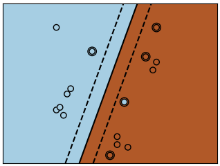
i) Linear kernel
>>> svc = svm.SVC(kernel='linear')
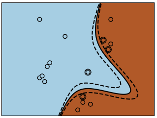
ii) Polynomial kernel
svc = svm.SVC(kernel='poly', degree=3)# degree: polynomial degree
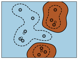
iii) RBF kernel (Radial Basis Function)
svc = svm.SVC(kernel='rbf')# gamma: inverse of size of# radial kernel
 :::info
Interactive example
:::info
Interactive example
See the SVM GUI to download svm_gui.py; add data points of both classes with right and left button, fit the model and change parameters and data.
:::
:::info
Exercise
Try classifying classes 1 and 2 from the iris dataset with SVMs, with the 2 first features. Leave out 10% of each class and test prediction performance on these observations. A solution can be downloaded here
Warning: the classes are ordered, do not leave out the last 10%, you would be testing on only one class.Hint: You can use the decision_function method on a grid to get intuitions.:::
iris = datasets.load_iris()X = iris.datay = iris.targetX = X[y != 0, :2]y = y[y != 0]
3、Model selection: choosing estimators and their parameters
📄 原文链接:https://scikit-learn.org/stable/tutorial/statistical_inference/model_selection.html
3.1 Score, and cross-validated scores
As we have seen, every estimator exposes a score method that can judge the quality of the fit (or the prediction) on new data. Bigger is better.
>>> from sklearn import datasets, svm>>> X_digits, y_digits = datasets.load_digits(return_X_y=True)>>> svc = svm.SVC(C=1, kernel='linear')>>> svc.fit(X_digits[:-100], y_digits[:-100]).score(X_digits[-100:], y_digits[-100:])0.98
To get a better measure of prediction accuracy (which we can use as a proxy for goodness of fit of the model), we can successively split the data in folds that we use for training and testing:
import numpy as npX_folds = np.array_split(X_digits, 3)y_folds = np.array_split(y_digits, 3)scores = list()for k in range(3):# We use 'list' to copy, in order to 'pop' later onX_train = list(X_folds)X_test = X_train.pop(k)X_train = np.concatenate(X_train)y_train = list(y_folds)y_test = y_train.pop(k)y_train = np.concatenate(y_train)scores.append(svc.fit(X_train, y_train).score(X_test, y_test))print(scores) # [0.934..., 0.956..., 0.939...]
3.2 Cross-validation generators
Scikit-learn has a collection of classes which can be used to generate lists of train/test indices for popular cross-validation strategies.
They expose a split method which accepts the input dataset to be split and yields the train/test set indices for each iteration of the chosen cross-validation strategy.
This example shows an example usage of the split method.
from sklearn.model_selection import KFold, cross_val_scoreX = ["a", "a", "a", "b", "b", "c", "c", "c", "c", "c"]k_fold = KFold(n_splits=5)for train_indices, test_indices in k_fold.split(X):print('Train: %s | test: %s' % (train_indices, test_indices))# Train: [2 3 4 5 6 7 8 9] | test: [0 1]# Train: [0 1 4 5 6 7 8 9] | test: [2 3]# Train: [0 1 2 3 6 7 8 9] | test: [4 5]# Train: [0 1 2 3 4 5 8 9] | test: [6 7]# Train: [0 1 2 3 4 5 6 7] | test: [8 9]
The cross-validation can then be performed easily:
[svc.fit(X_digits[train], y_digits[train]).score(X_digits[test], y_digits[test])for train, test in k_fold.split(X_digits)]# [0.963..., 0.922..., 0.963..., 0.963..., 0.930...]
The cross-validation score can be directly calculated using the cross_val_score helper. Given an estimator, the cross-validation object and the input dataset, the cross_val_score splits the data repeatedly into a training and a testing set, trains the estimator using the training set and computes the scores based on the testing set for each iteration of cross-validation.
By default the estimator’s score method is used to compute the individual scores.
Refer the metrics module to learn more on the available scoring methods.
>>> cross_val_score(svc, X_digits, y_digits, cv=k_fold, n_jobs=-1)array([0.96388889, 0.92222222, 0.9637883 , 0.9637883 , 0.93036212])
n_jobs=-1 means that the computation will be dispatched(迅速完成) on all the CPUs of the computer.
Alternatively, the scoring argument can be provided to specify an alternative scoring method.
>>> cross_val_score(svc, X_digits, y_digits, cv=k_fold, scoring='precision_macro')# array([0.96578289, 0.92708922, 0.96681476, 0.96362897, 0.93192644])
1) Cross-validation generators
| Methods | Description |
|---|---|
| KFold(n_splits, shuffle, random_state) | Splits it into K folds, trains on K-1 and then tests on the left-out. |
| StratifiedKFold(n_splits, shuffle, random_state) | Same as K-Fold but preserves(保留) the class distribution within each fold. |
| GroupKFold(n_splits) | Ensures that the same group is not in both testing and training sets. |
| ShuffleSplit(n_splits, test_size, train_size, random_state) | Generates train/test indices based on random permutation(组合). |
| StratifiedShuffleSplit | Same as shuffle split but preserves the class distribution within each iteration. |
| GroupShuffleSplit | Ensures that the same group is not in both testing and training sets. |
| LeaveOneGroupOut() | Takes a group array to group observations. |
| LeavePGroupsOut(n_groups) | Leave P groups out. |
| LeaveOneOut() | Leave one observation out. |
| LeavePOut(p) | Leave P observations out. |
| PredefinedSplit | Generates train/test indices based on predefined splits. |
:::info
Exercise
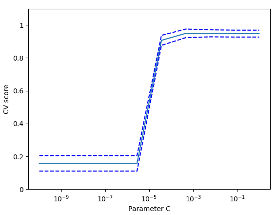
On the digits dataset, plot the cross-validation score of a SVC estimator with an linear kernel as a function of parameter C (use a logarithmic(对数的) grid of points, from 1 to 10).
Solution: Cross-validation on Digits Dataset Exercise
:::
import numpy as npfrom sklearn.model_selection import cross_val_scorefrom sklearn import datasets, svmimport matplotlib.pyplot as pltX, y = datasets.load_digits(return_X_y=True)svc = svm.SVC(kernel='linear')C_s = np.logspace(-10, 0, 10)scores = list()scores_std = list()for C in C_s:svc.C = Cthis_scores = cross_val_score(svc, X, y, n_jobs=1)scores.append(np.mean(this_scores))scores_std.append(np.std(this_scores))# Do the plottingplt.figure()plt.semilogx(C_s, scores)plt.semilogx(C_s, np.array(scores) + np.array(scores_std), 'b--')plt.semilogx(C_s, np.array(scores) - np.array(scores_std), 'b--')locs, labels = plt.yticks()plt.yticks(locs, list(map(lambda x: "%g" % x, locs)))plt.ylabel('CV score')plt.xlabel('Parameter C')plt.ylim(0, 1.1)plt.show()
3.3 Grid-search and cross-validated estimators
1) Grid-search
scikit-learn provides an object that, given data, computes the score during the fit of an estimator on a parameter grid and chooses the parameters to maximize the cross-validation score. This object takes an estimator during the construction and exposes an estimator API:
from sklearn.model_selection import GridSearchCV, cross_val_scoreCs = np.logspace(-6, -1, 10)clf = GridSearchCV(estimator=svc, param_grid=dict(C=Cs), n_jobs=-1)clf.fit(X_digits[:1000], y_digits[:1000])clf.best_score_ # 0.925...clf.best_estimator_.C # 0.0077...# Prediction performance on test set is not as good as on train setclf.score(X_digits[1000:], y_digits[1000:]) # 0.943...
By default, the GridSearchCV uses a 5-fold cross-validation. However, if it detects that a classifier is passed, rather than a regressor, it uses a stratified 5-fold.
:::info
Nested cross-validation
Two cross-validation loops are performed in parallel: one by the GridSearchCV estimator to set gamma and the other one by cross_val_score to measure the prediction performance of the estimator. The resulting scores are unbiased estimates of the prediction score on new data.
Warning:You cannot nest objects with parallel computing (n_jobs different than 1).
:::
>>> cross_val_score(clf, X_digits, y_digits)array([0.938..., 0.963..., 0.944...])
2) Cross-validated estimators
Cross-validation to set a parameter can be done more efficiently on an algorithm-by-algorithm basis. This is why, for certain estimators, scikit-learn exposes Cross-validation: evaluating estimator performance estimators that set their parameter automatically by cross-validation:
from sklearn import linear_model, datasetslasso = linear_model.LassoCV()X_diabetes, y_diabetes = datasets.load_diabetes(return_X_y=True)lasso.fit(X_diabetes, y_diabetes)# The estimator chose automatically its lambda:lasso.alpha_ # 0.00375...
These estimators are called similarly to their counterparts(对应的事物), with CV appended to their name.
:::info
Exercise
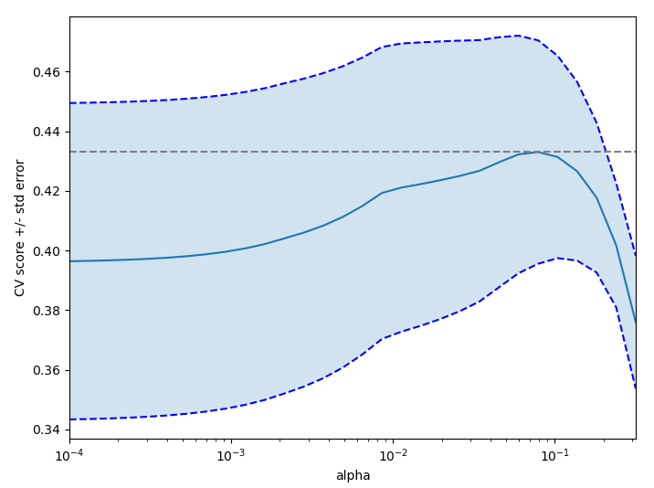
On the diabetes dataset, find the optimal regularization parameter alpha.
Bonus: How much can you trust the selection of alpha?
Solution: Cross-validation on diabetes Dataset Exercise
:::
import numpy as npimport matplotlib.pyplot as pltfrom sklearn import datasetsfrom sklearn.linear_model import LassoCVfrom sklearn.linear_model import Lassofrom sklearn.model_selection import KFoldfrom sklearn.model_selection import GridSearchCVX, y = datasets.load_diabetes(return_X_y=True)X = X[:150]y = y[:150]lasso = Lasso(random_state=0, max_iter=10000)alphas = np.logspace(-4, -0.5, 30)tuned_parameters = [{'alpha': alphas}]n_folds = 5clf = GridSearchCV(lasso, tuned_parameters, cv=n_folds, refit=False)clf.fit(X, y)scores = clf.cv_results_['mean_test_score']scores_std = clf.cv_results_['std_test_score']plt.figure().set_size_inches(8, 6)plt.semilogx(alphas, scores)# plot error lines showing +/- std. errors of the scoresstd_error = scores_std / np.sqrt(n_folds)plt.semilogx(alphas, scores + std_error, 'b--')plt.semilogx(alphas, scores - std_error, 'b--')# alpha=0.2 controls the translucency of the fill colorplt.fill_between(alphas, scores + std_error, scores - std_error, alpha=0.2)plt.ylabel('CV score +/- std error')plt.xlabel('alpha')plt.axhline(np.max(scores), linestyle='--', color='.5')plt.xlim([alphas[0], alphas[-1]])# ############################################################################## Bonus: how much can you trust the selection of alpha?# To answer this question we use the LassoCV object that sets its alpha# parameter automatically from the data by internal cross-validation (i.e. it# performs cross-validation on the training data it receives).# We use external cross-validation to see how much the automatically obtained# alphas differ across different cross-validation folds.lasso_cv = LassoCV(alphas=alphas, random_state=0, max_iter=10000)k_fold = KFold(3)print("Answer to the bonus question:", "how much can you trust the selection of alpha?")print("Alpha parameters maximising the generalization score on different")print("subsets of the data:")for k, (train, test) in enumerate(k_fold.split(X, y)):lasso_cv.fit(X[train], y[train])print("[fold {0}] alpha: {1:.5f}, score: {2:.5f}".format(k, lasso_cv.alpha_, lasso_cv.score(X[test], y[test])))print("Answer: Not very much since we obtained different alphas for different")print("subsets of the data and moreover, the scores for these alphas differ")print("quite substantially.")plt.show()
4、Unsupervised learning: seeking representations of the data
📄 原文链接:https://scikit-learn.org/stable/tutorial/statistical_inference/unsupervised_learning.html
4.1 Clustering: grouping observations together
:::info
The problem solved in clustering
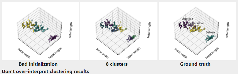
Given the iris dataset, if we knew that there were 3 types of iris, but did not have access to a taxonomist(分类学家) to label them: we could try a clustering task: split the observations into well-separated group called clusters.
:::
1) K-means clustering
Note that there exist a lot of different clustering criteria(标准) and associated algorithms. The simplest clustering algorithm is K-means.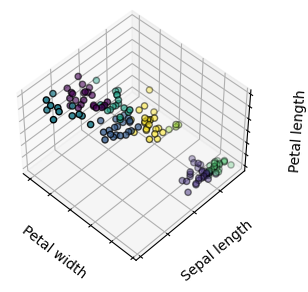
from sklearn import cluster, datasetsX_iris, y_iris = datasets.load_iris(return_X_y=True)k_means = cluster.KMeans(n_clusters=3)k_means.fit(X_iris)print(k_means.labels_[::10])# [1 1 1 1 1 0 0 0 0 0 2 2 2 2 2]print(y_iris[::10])# [0 0 0 0 0 1 1 1 1 1 2 2 2 2 2]
:::info Warning There is absolutely no guarantee of recovering a ground truth. First, choosing the right number of clusters is hard. Second, the algorithm is sensitive to initialization, and can fall into local minima, although scikit-learn employs several tricks to mitigate this issue.:::
:::info
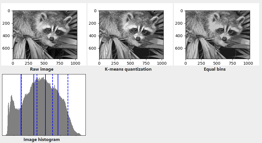
Application example: vector quantization
Clustering in general and KMeans, in particular, can be seen as a way of choosing a small number of exemplars(范例) to compress the information. The problem is sometimes known as vector quantization. For instance, this can be used to posterize(色彩分离) an image:
:::
import numpy as npimport scipy as spimport matplotlib.pyplot as pltfrom sklearn import clustertry: # SciPy >= 0.16 have face in miscfrom scipy.misc import faceface = face(gray=True)except ImportError:face = sp.face(gray=True)n_clusters = 5np.random.seed(0)X = face.reshape((-1, 1)) # We need an (n_sample, n_feature) arrayk_means = cluster.KMeans(n_clusters=n_clusters, n_init=4)k_means.fit(X)values = k_means.cluster_centers_.squeeze()labels = k_means.labels_# create an array from labels and valuesface_compressed = np.choose(labels, values)face_compressed.shape = face.shapevmin = face.min()vmax = face.max()# original faceplt.figure(1, figsize=(3, 2.2))plt.imshow(face, cmap=plt.cm.gray, vmin=vmin, vmax=256)# compressed faceplt.figure(2, figsize=(3, 2.2))plt.imshow(face_compressed, cmap=plt.cm.gray, vmin=vmin, vmax=vmax)# equal bins faceregular_values = np.linspace(0, 256, n_clusters + 1)regular_labels = np.searchsorted(regular_values, face) - 1regular_values = .5 * (regular_values[1:] + regular_values[:-1]) # meanregular_face = np.choose(regular_labels.ravel(), regular_values, mode="clip")regular_face.shape = face.shapeplt.figure(3, figsize=(3, 2.2))plt.imshow(regular_face, cmap=plt.cm.gray, vmin=vmin, vmax=vmax)# histogramplt.figure(4, figsize=(3, 2.2))plt.clf()plt.axes([.01, .01, .98, .98])plt.hist(X, bins=256, color='.5', edgecolor='.5')plt.yticks(())plt.xticks(regular_values)values = np.sort(values)for center_1, center_2 in zip(values[:-1], values[1:]):plt.axvline(.5 * (center_1 + center_2), color='b')for center_1, center_2 in zip(regular_values[:-1], regular_values[1:]):plt.axvline(.5 * (center_1 + center_2), color='b', linestyle='--')plt.show()
2) Hierarchical agglomerative clustering: Ward
A Hierarchical clustering method is a type of cluster analysis that aims to build a hierarchy(层次) of clusters. In general, the various approaches of this technique are either:
- Agglomerative(凝聚) - bottom-up approaches: each observation starts in its own cluster, and clusters are iteratively merged in such a way to minimize a linkage(连接) criterion. This approach is particularly interesting when the clusters of interest are made of only a few observations. When the number of clusters is large, it is much more computationally efficient than k-means.
- Divisive(分裂) - top-down approaches: all observations start in one cluster, which is iteratively split as one moves down the hierarchy. For estimating large numbers of clusters, this approach is both slow (due to all observations starting as one cluster, which it splits recursively) and statistically ill-posed(不适应的).
3) Connectivity-constrained clustering
With agglomerative clustering, it is possible to specify which samples can be clustered together by giving a connectivity graph. Graphs in scikit-learn are represented by their adjacency matrix. Often, a sparse matrix is used. This can be useful, for instance, to retrieve(检索数据) connected regions (sometimes also referred to(提到) as connected components) when clustering an image.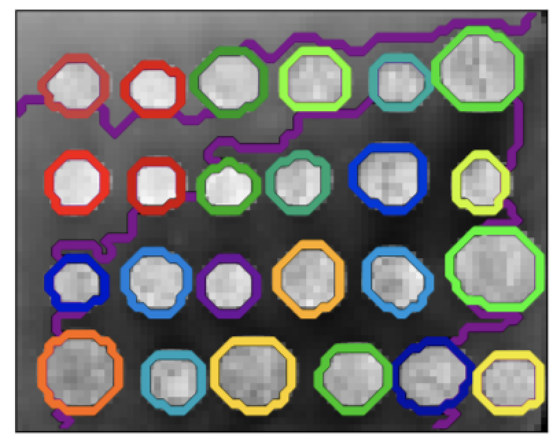 ```python
import time as time
import numpy as np
import matplotlib.pyplot as plt
import skimage
from skimage.data import coins
from skimage.transform import rescale
from scipy.ndimage.filters import gaussian_filter
from sklearn.feature_extraction.image import grid_to_graph
from sklearn.cluster import AgglomerativeClustering
from sklearn.utils.fixes import parse_version
```python
import time as time
import numpy as np
import matplotlib.pyplot as plt
import skimage
from skimage.data import coins
from skimage.transform import rescale
from scipy.ndimage.filters import gaussian_filter
from sklearn.feature_extraction.image import grid_to_graph
from sklearn.cluster import AgglomerativeClustering
from sklearn.utils.fixes import parse_version
these were introduced in skimage-0.14
if parseversion(skimage._version) >= parse_version(‘0.14’): rescale_params = {‘anti_aliasing’: False, ‘multichannel’: False} else: rescale_params = {}
#
Generate data
orig_coins = coins()
Resize it to 20% of the original size to speed up the processing
Applying a Gaussian filter for smoothing prior to down-scaling
reduces aliasing artifacts.
smoothened_coins = gaussian_filter(orig_coins, sigma=2) rescaled_coins = rescale(smoothened_coins, 0.2, mode=”reflect”, **rescale_params)
X = np.reshape(rescaled_coins, (-1, 1))
#
Define the structure A of the data. Pixels connected to their neighbors.
connectivity = grid_to_graph(*rescaled_coins.shape)
#
Compute clustering
print(“Compute structured hierarchical clustering…”) st = time.time() nclusters = 27 # number of regions ward = AgglomerativeClustering(n_clusters=n_clusters, linkage=’ward’, connectivity=connectivity) ward.fit(X) label = np.reshape(ward.labels, rescaled_coins.shape) print(“Elapsed time: “, time.time() - st) print(“Number of pixels: “, label.size) print(“Number of clusters: “, np.unique(label).size)
#
Plot the results on an image
plt.figure(figsize=(5, 5)) plt.imshow(rescaled_coins, cmap=plt.cm.gray)
for l in range(n_clusters): plt.contour(label == l, colors=[plt.cm.nipy_spectral(l / float(n_clusters)), ])
plt.xticks(()) plt.yticks(()) plt.show()
We need a vectorized version of the image. `'rescaled_coins'` is a down-scaled version of the coins image to speed up the process:```pythonfrom sklearn.feature_extraction import grid_to_graphconnectivity = grid_to_graph(*rescaled_coins.shape)
Define the graph structure of the data. Pixels connected to their neighbors:
n_clusters = 27 # number of regionsfrom sklearn.cluster import AgglomerativeClusteringward = AgglomerativeClustering(n_clusters=n_clusters, linkage='ward', connectivity=connectivity)ward.fit(X)label = np.reshape(ward.labels_, rescaled_coins.shape)
4) Feature agglomeration
We have seen that sparsity could be used to mitigate(缓和) the curse of dimensionality, i.e an insufficient(不足的) amount of observations compared to the number of features. Another approach is to merge together similar features: feature agglomeration. This approach can be implemented by clustering in the feature direction, in other words clustering the transposed(变形的) data.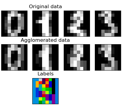
import numpy as npimport matplotlib.pyplot as pltfrom sklearn import datasets, clusterfrom sklearn.feature_extraction.image import grid_to_graphdigits = datasets.load_digits()images = digits.imagesX = np.reshape(images, (len(images), -1))connectivity = grid_to_graph(*images[0].shape)agglo = cluster.FeatureAgglomeration(connectivity=connectivity, n_clusters=32)agglo.fit(X)X_reduced = agglo.transform(X)X_restored = agglo.inverse_transform(X_reduced)images_restored = np.reshape(X_restored, images.shape)plt.figure(1, figsize=(4, 3.5))plt.clf()plt.subplots_adjust(left=.01, right=.99, bottom=.01, top=.91)for i in range(4):plt.subplot(3, 4, i + 1)plt.imshow(images[i], cmap=plt.cm.gray, vmax=16, interpolation='nearest')plt.xticks(())plt.yticks(())if i == 1:plt.title('Original data')plt.subplot(3, 4, 4 + i + 1)plt.imshow(images_restored[i], cmap=plt.cm.gray, vmax=16,interpolation='nearest')if i == 1:plt.title('Agglomerated data')plt.xticks(())plt.yticks(())plt.subplot(3, 4, 10)plt.imshow(np.reshape(agglo.labels_, images[0].shape),interpolation='nearest', cmap=plt.cm.nipy_spectral)plt.xticks(())plt.yticks(())plt.title('Labels')plt.show()
:::info
transform** and inverse_transform methods**
Some estimators expose a transform method, for instance to reduce the dimensionality of the dataset.
:::
5、Decompositions: from a signal to components and loadings
:::info
Components and loadings
If X is our multivariate data, then the problem that we are trying to solve is to rewrite it on a different observational basis: we want to learn loadings L and a set of components C such that X = L C. Different criteria exist to choose the components
:::
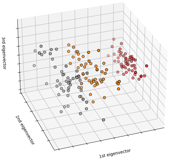
5.1 Principal component analysis: PCA
Principal component analysis (PCA) selects the successive components that explain the maximum variance in the signal.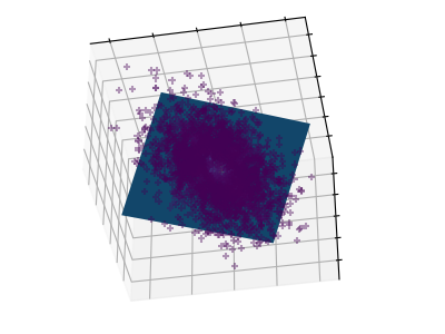
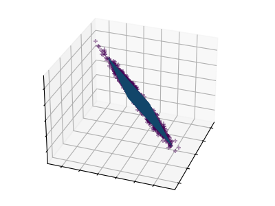
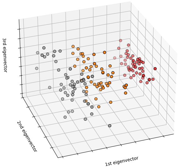
The point cloud spanned(贯穿) by the observations above is very flat in one direction: one of the three univariate(单变量的) features can almost be exactly computed using the other two. PCA finds the directions in which the data is not flat
When used to _transform data, PCA can reduce the dimensionality of the data by projecting on(投射) a principal subspace.
# Create a signal with only 2 useful dimensionsx1 = np.random.normal(size=100)x2 = np.random.normal(size=100)x3 = x1 + x2X = np.c_[x1, x2, x3]from sklearn import decompositionpca = decomposition.PCA()pca.fit(X)print(pca.explained_variance_)# [ 2.18565811e+00 1.19346747e+00 8.43026679e-32]# As we can see, only the 2 first components are usefulpca.n_components = 2X_reduced = pca.fit_transform(X)X_reduced.shape # (100, 2)
5.2 Independent Component Analysis: ICA
Independent component analysis (ICA) selects components so that the distribution of their loadings carries a maximum amount of independent information. It is able to recover non-Gaussian independent signals: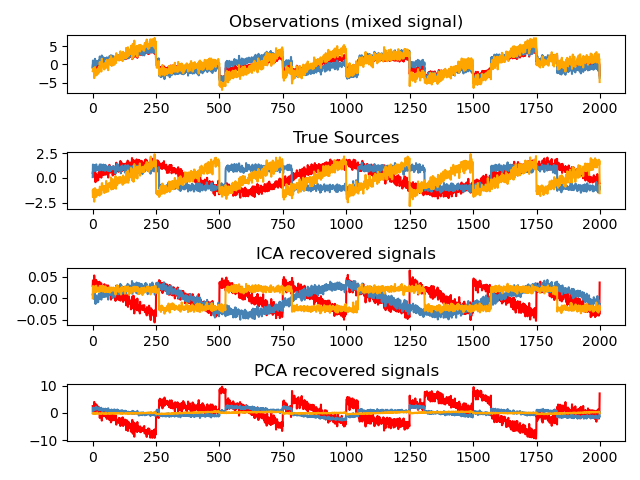
import numpy as npimport matplotlib.pyplot as pltfrom scipy import signalfrom sklearn.decomposition import FastICA, PCA# ############################################################################## Generate sample datanp.random.seed(0)n_samples = 2000time = np.linspace(0, 8, n_samples)s1 = np.sin(2 * time) # Signal 1 : sinusoidal signals2 = np.sign(np.sin(3 * time)) # Signal 2 : square signals3 = signal.sawtooth(2 * np.pi * time) # Signal 3: saw tooth signalS = np.c_[s1, s2, s3]S += 0.2 * np.random.normal(size=S.shape) # Add noiseS /= S.std(axis=0) # Standardize data# Mix dataA = np.array([[1, 1, 1], [0.5, 2, 1.0], [1.5, 1.0, 2.0]]) # Mixing matrixX = np.dot(S, A.T) # Generate observations# Compute ICAica = FastICA(n_components=3)S_ = ica.fit_transform(X) # Reconstruct signalsA_ = ica.mixing_ # Get estimated mixing matrix# We can `prove` that the ICA model applies by reverting the unmixing.assert np.allclose(X, np.dot(S_, A_.T) + ica.mean_)# For comparison, compute PCApca = PCA(n_components=3)H = pca.fit_transform(X) # Reconstruct signals based on orthogonal components# ############################################################################## Plot resultsplt.figure()models = [X, S, S_, H]names = ['Observations (mixed signal)','True Sources','ICA recovered signals','PCA recovered signals']colors = ['red', 'steelblue', 'orange']for ii, (model, name) in enumerate(zip(models, names), 1):plt.subplot(4, 1, ii)plt.title(name)for sig, color in zip(model.T, colors):plt.plot(sig, color=color)plt.tight_layout()plt.show()
6、Putting it all together
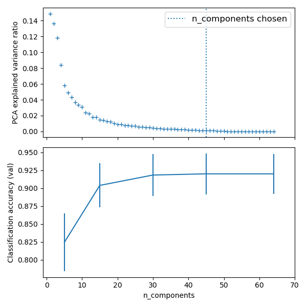
6.1 Pipelining
We have seen that some estimators can transform data and that some estimators can predict variables. We can also create combined estimators:
import matplotlib.pyplot as pltimport pandas as pdfrom sklearn import datasetsfrom sklearn.decomposition import PCAfrom sklearn.linear_model import LogisticRegressionfrom sklearn.pipeline import Pipelinefrom sklearn.model_selection import GridSearchCV# Define a pipeline to search for the best combination of PCA truncation# and classifier regularization.pca = PCA()# set the tolerance to a large value to make the example fasterlogistic = LogisticRegression(max_iter=10000, tol=0.1)pipe = Pipeline(steps=[('pca', pca), ('logistic', logistic)])X_digits, y_digits = datasets.load_digits(return_X_y=True)# Parameters of pipelines can be set using ‘__’ separated parameter names:param_grid = {'pca__n_components': [5, 15, 30, 45, 64],'logistic__C': np.logspace(-4, 4, 4),}search = GridSearchCV(pipe, param_grid, n_jobs=-1)search.fit(X_digits, y_digits)print("Best parameter (CV score=%0.3f):" % search.best_score_)print(search.best_params_)# Plot the PCA spectrumpca.fit(X_digits)fig, (ax0, ax1) = plt.subplots(nrows=2, sharex=True, figsize=(6, 6))ax0.plot(np.arange(1, pca.n_components_ + 1),pca.explained_variance_ratio_, '+', linewidth=2)ax0.set_ylabel('PCA explained variance ratio')ax0.axvline(search.best_estimator_.named_steps['pca'].n_components,linestyle=':', label='n_components chosen')ax0.legend(prop=dict(size=12))
6.2 Face recognition with eigenfaces
The dataset used in this example is a preprocessed excerpt of the “Labeled Faces in the Wild”, also known as LFW: http://vis-www.cs.umass.edu/lfw/lfw-funneled.tgz (233MB)
"""===================================================Faces recognition example using eigenfaces and SVMs===================================================The dataset used in this example is a preprocessed excerpt of the"Labeled Faces in the Wild", aka LFW_:http://vis-www.cs.umass.edu/lfw/lfw-funneled.tgz (233MB).. _LFW: http://vis-www.cs.umass.edu/lfw/Expected results for the top 5 most represented people in the dataset:================== ============ ======= ========== =======precision recall f1-score support================== ============ ======= ========== =======Ariel Sharon 0.67 0.92 0.77 13Colin Powell 0.75 0.78 0.76 60Donald Rumsfeld 0.78 0.67 0.72 27George W Bush 0.86 0.86 0.86 146Gerhard Schroeder 0.76 0.76 0.76 25Hugo Chavez 0.67 0.67 0.67 15Tony Blair 0.81 0.69 0.75 36avg / total 0.80 0.80 0.80 322================== ============ ======= ========== ======="""import loggingimport matplotlib.pyplot as pltfrom time import timefrom sklearn.model_selection import train_test_splitfrom sklearn.model_selection import GridSearchCVfrom sklearn.datasets import fetch_lfw_peoplefrom sklearn.metrics import classification_reportfrom sklearn.metrics import confusion_matrixfrom sklearn.decomposition import PCAfrom sklearn.svm import SVC# Display progress logs on stdoutlogging.basicConfig(level=logging.INFO, format='%(asctime)s %(message)s')# ############################################################################## Download the data, if not already on disk and load it as numpy arrayslfw_people = fetch_lfw_people(min_faces_per_person=70, resize=0.4)# introspect the images arrays to find the shapes (for plotting)n_samples, h, w = lfw_people.images.shape# for machine learning we use the 2 data directly (as relative pixel# positions info is ignored by this model)X = lfw_people.datan_features = X.shape[1]# the label to predict is the id of the persony = lfw_people.targettarget_names = lfw_people.target_namesn_classes = target_names.shape[0]print("Total dataset size:")print("n_samples: %d" % n_samples)print("n_features: %d" % n_features)print("n_classes: %d" % n_classes)# ############################################################################## Split into a training set and a test set using a stratified k fold# split into a training and testing setX_train, X_test, y_train, y_test = train_test_split(X, y, test_size=0.25, random_state=42)# ############################################################################## Compute a PCA (eigenfaces) on the face dataset (treated as unlabeled# dataset): unsupervised feature extraction / dimensionality reductionn_components = 150print("Extracting the top %d eigenfaces from %d faces" % (n_components, X_train.shape[0]))t0 = time()pca = PCA(n_components=n_components, svd_solver='randomized', whiten=True).fit(X_train)print("done in %0.3fs" % (time() - t0))eigenfaces = pca.components_.reshape((n_components, h, w))print("Projecting the input data on the eigenfaces orthonormal basis")t0 = time()X_train_pca = pca.transform(X_train)X_test_pca = pca.transform(X_test)print("done in %0.3fs" % (time() - t0))# ############################################################################## Train a SVM classification modelprint("Fitting the classifier to the training set")t0 = time()param_grid = {'C': [1e3, 5e3, 1e4, 5e4, 1e5],'gamma': [0.0001, 0.0005, 0.001, 0.005, 0.01, 0.1],}clf = GridSearchCV(SVC(kernel='rbf', class_weight='balanced'), param_grid)clf = clf.fit(X_train_pca, y_train)print("done in %0.3fs" % (time() - t0))print("Best estimator found by grid search:")print(clf.best_estimator_)# ############################################################################## Quantitative evaluation of the model quality on the test setprint("Predicting people's names on the test set")t0 = time()y_pred = clf.predict(X_test_pca)print("done in %0.3fs" % (time() - t0))print(classification_report(y_test, y_pred, target_names=target_names))print(confusion_matrix(y_test, y_pred, labels=range(n_classes)))# ############################################################################## Qualitative evaluation of the predictions using matplotlibdef plot_gallery(images, titles, h, w, n_row=3, n_col=4):"""Helper function to plot a gallery of portraits"""plt.figure(figsize=(1.8 * n_col, 2.4 * n_row))plt.subplots_adjust(bottom=0, left=.01, right=.99, top=.90, hspace=.35)for i in range(n_row * n_col):plt.subplot(n_row, n_col, i + 1)plt.imshow(images[i].reshape((h, w)), cmap=plt.cm.gray)plt.title(titles[i], size=12)plt.xticks(())plt.yticks(())# plot the result of the prediction on a portion of the test setdef title(y_pred, y_test, target_names, i):pred_name = target_names[y_pred[i]].rsplit(' ', 1)[-1]true_name = target_names[y_test[i]].rsplit(' ', 1)[-1]return 'predicted: %s\ntrue: %s' % (pred_name, true_name)prediction_titles = [title(y_pred, y_test, target_names, i)for i in range(y_pred.shape[0])]plot_gallery(X_test, prediction_titles, h, w)# plot the gallery of the most significative eigenfaceseigenface_titles = ["eigenface %d" % i for i in range(eigenfaces.shape[0])]plot_gallery(eigenfaces, eigenface_titles, h, w)plt.show()

若有收获,就点个赞吧
0 人点赞
