总结
1.在 Java1.7 中,HashMap 的数据结构为数组 + 单向链表。Java1.8 中变成了数组 + 单向链表 + 红黑树。
2.在 Java1.7 中,插入链表节点使用头插法。Java1.8 中变成了尾插法。
3.在 java 1.8 中,Entry 被 Node 替代 (换了一个马甲。
Java1.8 的 hash() 中,将 hash 值高位(前 16 位)参与到取模的运算中,使得计算结果的不确定性增强,降低发生哈希碰撞的概率。
JDK1.7中
使用一个 Entry 数组来存储数据,用key的 hashcode 取模来决定key会被放到数组里的位置,如果 hashcode 相同,或者 hashcode 取模后的结果相同( hash collision ),那么这些 key 会被定位到 Entry 数组的同一个格子里,这些 key 会形成一个链表。
在 hashcode 特别差的情况下,比方说所有key的 hashcode 都相同,这个链表可能会很长,那么 put/get 操作都可能需要遍历这个链表,也就是说时间复杂度在最差情况下会退化到 O(n)
JDK1.8中
使用一个 Node 数组来存储数据,但这个 Node 可能是链表结构,也可能是红黑树结构
- 如果插入的 key 的 hashcode 相同,那么这些key也会被定位到 Node 数组的同一个格子里。
- 如果同一个格子里的key不超过8个,使用链表结构存储。
- 如果超过了8个,那么会调用 treeifyBin 函数,将链表转换为红黑树。
那么即使 hashcode 完全相同,由于红黑树的特点,查找某个特定元素,也只需要O(log n)的开销也就是说put/get的操作的时间复杂度最差只有 O(log n)
听起来挺不错,但是真正想要利用 JDK1.8 的好处,有一个限制:key的对象,必须正确的实现了 Compare 接口
如果没有实现 Compare 接口,或者实现得不正确(比方说所有 Compare 方法都返回0)那 JDK1.8 的 HashMap 其实还是慢于 JDK1.7 的
简单的测试数据如下:
向 HashMap 中 put/get 1w 条 hashcode 相同的对象
JDK1.7: put 0.26s , get 0.55s
JDK1.8 (未实现 Compare 接口): put 0.92s , get 2.1s
但是如果正确的实现了 Compare 接口,那么 JDK1.8 中的 HashMap 的性能有巨大提升,这次 put/get 100W条hashcode 相同的对象
JDK1.8 (正确实现 Compare 接口,): put/get 大概开销都在320 ms 左右
一、数据结构
在 Java1.7 中,HashMap 的数据结构为数组 + 单向链表。Java1.8 中变成了数组 + 单向链表 + 红黑树。
jdk1.7.0_80
插入 key-value 时主要有两个步骤:
- 根据 key 的hash值,找到 key-value 要存放的桶(bucketIndex),也就是对应数组元素的下标。
- 当不同 key 发生哈希冲突时,key-value 会以单向链表的形式存储,并使用头插法插入。
哈希冲突:
-key 相同
-key 不同,hash 值相同
-key 不同,hash 值不同,hash 值取模后相同
`// put方法public V put(K key, V value) {if (table == EMPTY_TABLE) {// 初始化tableinflateTable(threshold);}if (key == null)return putForNullKey(value);int hash = hash(key);// 计算对应数组元素的下标int i = indexFor(hash, table.length);// 遍历数组中的链表,key存在时更新valuefor (Entry<K,V> e = table[i]; e != null; e = e.next) {Object k;if (e.hash == hash && ((k = e.key) == key || key.equals(k))) {V oldValue = e.value;e.value = value;e.recordAccess(this);return oldValue;}}modCount++;// key不存在,插入key-valueaddEntry(hash, key, value, i);return null;}// 初始化table,确保table的大小是2的次幂private void inflateTable(int toSize) {// Find a power of 2 >= toSizeint capacity = roundUpToPowerOf2(toSize);threshold = (int) Math.min(capacity * loadFactor, MAXIMUM_CAPACITY + 1);table = new Entry[capacity];initHashSeedAsNeeded(capacity);}// 插入key-valuevoid addEntry(int hash, K key, V value, int bucketIndex) {// HashMap容量超过阀值,进行扩容if ((size >= threshold) && (null != table[bucketIndex])) {resize(2 * table.length);hash = (null != key) ? hash(key) : 0;bucketIndex = indexFor(hash, table.length);}// 插入key-valuecreateEntry(hash, key, value, bucketIndex);}`
    // 头插法
    void createEntry(int hash, K key, V value, int bucketIndex) {
        Entry<K,V> e = table[bucketIndex];
        table[bucketIndex] = new Entry<>(hash, key, value, e);
        size++;
    }

    Entry(int h, K k, V v, Entry<K,V> n) {
        value = v;
        next = n;
        key = k;
        hash = h;
    }
jdk1.8.0_231
插入 key-value 时,增加了一个链表与红黑树之间转换的步骤 -> 当链表节点数量达到树化阀值(TREEIFY_THRESHOLD)时,链表就会转化为红黑树。
需要注意的是,当红黑树的节点数量减少到 UNTREEIFY_THRESHOLD 时,红黑树又会转化为单向链表。
 `// put方法
    public V put(K key, V value) {
        return putVal(hash(key), key, value, false, true);
    }

    final V putVal(int hash, K key, V value, boolean onlyIfAbsent,
                   boolean evict) {
        Node<K,V>[] tab; Node<K,V> p; int n, i;
        // 初始化table
        if ((tab = table) == null || (n = tab.length) == 0)
            n = (tab = resize()).length;
        // key是第一个插入对应的桶,直接插入
        if ((p = tab[i = (n - 1) & hash]) == null)
            tab[i] = newNode(hash, key, value, null);
        else {
            Node<K,V> e; K k;
            // key相同时,更新value
            if (p.hash == hash &&
                ((k = p.key) == key || (key != null && key.equals(k))))
                e = p;
            // 当前桶中是树节点时,将key-value插入树中
            else if (p instanceof TreeNode)
                e = ((TreeNode<K,V>)p).putTreeVal(this, tab, hash, key, value);
            // 当前桶中时单向链表时
            else {
                // 遍历链表,binCount为节点数量
                for (int binCount = 0; ; ++binCount) {
                    // 尾插法将key-value插入链表
                    if ((e = p.next) == null) {
                        p.next = newNode(hash, key, value, null);
                        // 链表节点数量即将到达树化阀值时,将链表转换为红黑树
                        if (binCount >= TREEIFY_THRESHOLD - 1) // -1 for 1st
                            treeifyBin(tab, hash);
                        break;
                    }
                    if (e.hash == hash &&
                        ((k = e.key) == key || (key != null && key.equals(k))))
                        break;
                    p = e;
                }
            }
            if (e != null) { // existing mapping for key
                V oldValue = e.value;
                if (!onlyIfAbsent || oldValue == null)
                    e.value = value;
                afterNodeAccess(e);
                return oldValue;
            }
        }
        ++modCount;
        if (++size > threshold)
            resize();
        afterNodeInsertion(evict);
        return null;
    }`
为什么
链表的增删效率高,查询效率低。
红黑树的增删效率低,查询效率高。
当 HashMap 中存储的数据越来越多,链表越来越长,查询数据效率就不太理想。使用红黑树代替链表,虽然牺牲了部分增删的性能,却提升了查询的性能。
链表查询的时间复杂度为 O(n),红黑树查询的时间复杂度为 O(logn)。
二、链表插入节点的方式
在 Java1.7 中,插入链表节点使用头插法。Java1.8 中变成了尾插法。
jdk1.7.0_80
 `void resize(int newCapacity) {
        Entry[] oldTable = table;
        int oldCapacity = oldTable.length;
        if (oldCapacity == MAXIMUM_CAPACITY) {
            threshold = Integer.MAX_VALUE;
            return;
        }

        Entry[] newTable = new Entry[newCapacity];
        transfer(newTable, initHashSeedAsNeeded(newCapacity));
        table = newTable;
        threshold = (int)Math.min(newCapacity * loadFactor, MAXIMUM_CAPACITY + 1);
    }

    // 复制HashMap中元素
    void transfer(Entry[] newTable, boolean rehash) {
        int newCapacity = newTable.length;
        // 遍历链表
        for (Entry<K,V> e : table) {
            while(null != e) {
                Entry<K,V> next = e.next;
                if (rehash) {
                    e.hash = null == e.key ? 0 : hash(e.key);
                }
                int i = indexFor(e.hash, newCapacity);
                // 插入新HashMap的链表中
                // 由于使用尾插法,复制后的新链表相对于原来的链表来说是倒序的
                e.next = newTable[i];
                newTable[i] = e;
                e = next;
            }
        }
    }`
jdk1.8.0_231
 `final Node<K,V>[] resize() {
        ……
        @SuppressWarnings({"rawtypes","unchecked"})
        Node<K,V>[] newTab = (Node<K,V>[])new Node[newCap];
        table = newTab;
        if (oldTab != null) {
            for (int j = 0; j < oldCap; ++j) {
                Node<K,V> e;
                if ((e = oldTab[j]) != null) {
                    oldTab[j] = null;
                    // 复制单节点
                    if (e.next == null)
                        newTab[e.hash & (newCap - 1)] = e;
                    // 复制树节点
                    else if (e instanceof TreeNode)
                        ((TreeNode<K,V>)e).split(this, newTab, j, oldCap);
                    // 复制链表节点
                    else { // preserve order
                        // resize前原本存在的桶(bucket)中的链表
                        Node<K,V> loHead = null, loTail = null;
                        // resize后扩容产生的桶(bucket)中的链表
                        Node<K,V> hiHead = null, hiTail = null;
                        Node<K,V> next;
                        do {
                            next = e.next;
                            // resize前后,桶的位置未变化
                            // 尾插法插入链表
                            if ((e.hash & oldCap) == 0) {
                                if (loTail == null)
                                    loHead = e;
                                else
                                    loTail.next = e;
                                loTail = e;
                            }
                            // resize后新产生的桶
                            // 尾插法插入链表
                            else {
                                if (hiTail == null)
                                    hiHead = e;
                                else
                                    hiTail.next = e;
                                hiTail = e;
                            }
                        } while ((e = next) != null);
                        if (loTail != null) {
                            loTail.next = null;
                            newTab[j] = loHead;
                        }
                        if (hiTail != null) {
                            hiTail.next = null;
                            newTab[j + oldCap] = hiHead;
                        }
                    }
                }
            }
        }
        return newTab;
    }`
为什么
头插法主要存在的问题是:并发下调用 transfer() 方法,可能会导致链表死循环,以及数据的丢失。
    void transfer(Entry[] newTable, boolean rehash) {
        int newCapacity = newTable.length;
        for (Entry<K,V> e : table) {
            while(null != e) {
                Entry<K,V> next = e.next;
                if (rehash) {
                    e.hash = null == e.key ? 0 : hash(e.key);
                }
                int i = indexFor(e.hash, newCapacity);
                e.next = newTable[i];
                newTable[i] = e;
                e = next;
            }
        }
    }
假设扩容前的 HashMap 是这样的: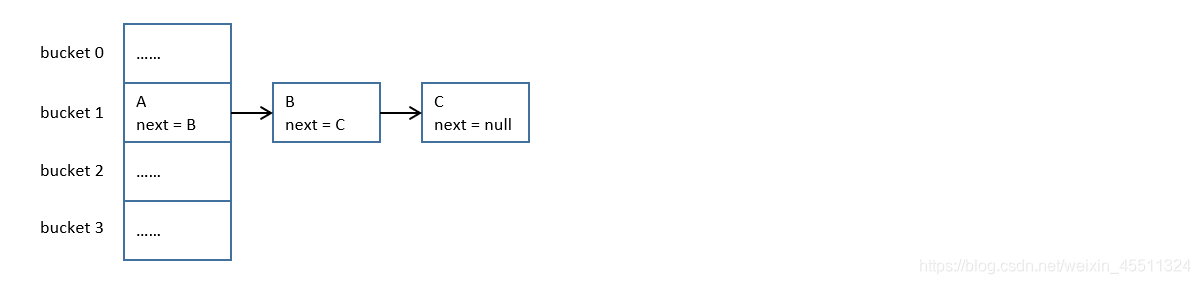
第一个线程插入 key-value,引起扩容。在 newTable[i] = e; 语句执行前,cpu 时间片用完,线程挂起。
第二个线程获得 cpu 时间片锁,也进行 HashMap 的扩容,结果如下。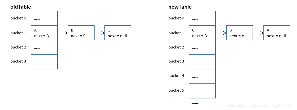
这时第一个线程重新获得 cpu 时间片锁,继续执行。只是第二个线程执行后,已经形成了 C→B→A 的链表了。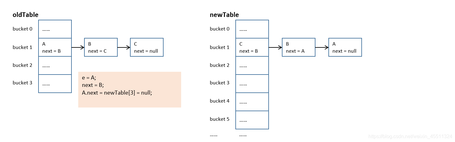
第一个线程走完当前的循环(e = A;next = B),结果为: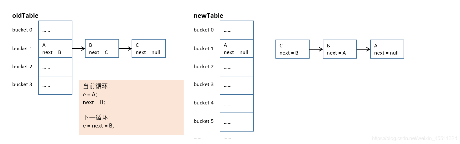
第一个线程继续下一个循环(e = B;next = A),结果为: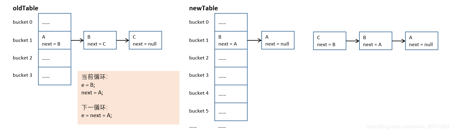
第一个线程继续下一个循环(e = A;next = null),结果为:
此时已经形成 A 和 B 的循环链表,调用 get() 方法时会进入死循环;同时 C 已经丢失,不存储在 HashMap 中。
三、hash 函数
Java1.8 的 hash() 中,将 hash 值高位(前 16 位)参与到取模的运算中,使得计算结果的不确定性增强,降低发生哈希碰撞的概率。
jdk1.7.0_80
    final int hash(Object k) {
        int h = hashSeed;
        if (0 != h && k instanceof String) {
            return sun.misc.Hashing.stringHash32((String) k);
        }

        h ^= k.hashCode();

        // This function ensures that hashCodes that differ only by
        // constant multiples at each bit position have a bounded
        // number of collisions (approximately 8 at default load factor).
        h ^= (h >>> 20) ^ (h >>> 12);
        return h ^ (h >>> 7) ^ (h >>> 4);
    }
jdk1.8.0_231
    static final int hash(Object key) {
        int h;
        return (key == null) ? 0 : (h = key.hashCode()) ^ (h >>> 16);
    }
四、扩容时计算数组元素下标的算法
jdk1.7.0_80
    static int indexFor(int h, int length) {
        // assert Integer.bitCount(length) == 1 : "length must be a non-zero power of 2";
        return h & (length-1);
    }
jdk1.8.0_231
do {
    next = e.next;
    // resize前后,桶的位置未变化
    // 尾插法插入链表
    if ((e.hash & oldCap) == 0) {
        if (loTail == null)
            loHead = e;
        else
            loTail.next = e;
        loTail = e;
    }
    // resize后新产生的桶
    // 尾插法插入链表
    else {
        if (hiTail == null)
            hiHead = e;
        else
            hiTail.next = e;
        hiTail = e;
    }
} while ((e = next) != null);
为什么
实际上,我们很容易发现规律:
原本在同一个桶中的 key,在扩容后,HashMap 容量翻倍,再去取模,实际上是需要高一位来参与计算的。(e.hash & oldCap) == 0 就是进行了这样的计算。
当高位是 0 时,newBucketIndex = oldBucketIndex,此时元素还是存放在原来的桶中;
当高位是 1 时,newBucketIndex = oldBucketIndex + oldTable.length,这时元素需要移动到扩容产生的桶中。
原文:
https://blog.csdn.net/weixin_45511324/article/details/104540826

若有收获,就点个赞吧
0 人点赞
