张量的简介与创建
这部分内容介绍 pytorch 中的数据结构——Tensor,Tensor 是 PyTorch 中最基础的概念,其参与了整个运算过程,主要介绍张量的概念和属性,如 data, device, dtype 等,并介绍 tensor 的基本创建方法,如直接创建、依数值创建和依概率分布创建等。
张量简介
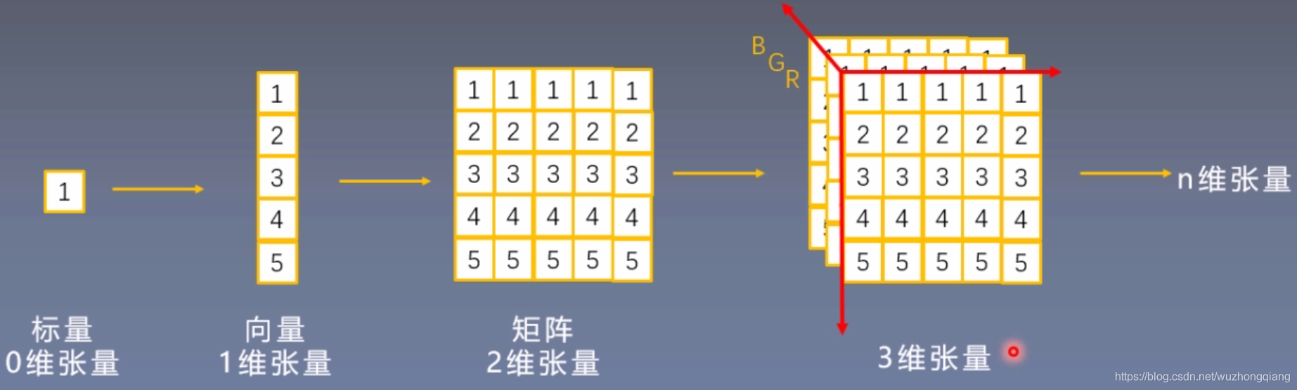
张量的基本概念
Tensor 与 Variable
在 Pytorch0.4.0 版本之后其实 Variable 已经并入 Tensor, 但是 Variable 这个数据类型的了解,对于理解张量来说很有帮助, 这到底是个什么呢?
Variable 是 torch.autograd 中的数据类型。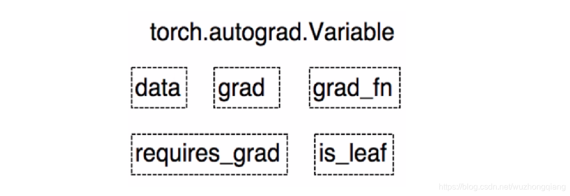
Variable 有下面的 5 个属性:
- data: 被包装的 Tensor
- grad: data 的梯度
- grad_fn: fn 表示 function 的意思,记录我么创建的创建张量时用到的方法,比如说加法,乘法,这个操作在求导过程需要用到,Tensor 的 Function, 是自动求导的关键
- requires_grad: 指示是否需要梯度, 有的不需要梯度
- is_leaf: 指示是否是叶子节点(张量)
这些属性都是为了张量的自动求导而设置的, 从 Pytorch0.4.0 版开始,Variable 并入了 Tensor, 看看张量里面的属性: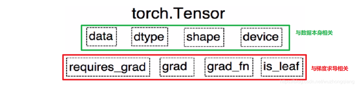
可以发现,如今版本里面的 Tensor 共有 8 个属性,上面四个与数据本身相关,下面四个与梯度求导相关。 其中有五个是 Variable 并入过来的, 这些含义就不解释了, 而还有三个属性没有说:
- dtype: 张量的数据类型, 如 torch.FloatTensor, torch.cuda.FloatTensor, 用的最多的一般是 float32 和 int64(torch.long)
- shape: 张量的形状, 如 (64, 3, 224, 224)
- device: 张量所在的设备, GPU/CPU, 张量放在 GPU 上才能使用加速。
张量的创建
直接创建张量
torch.Tensor(): 功能: 从 data 创建 Tensor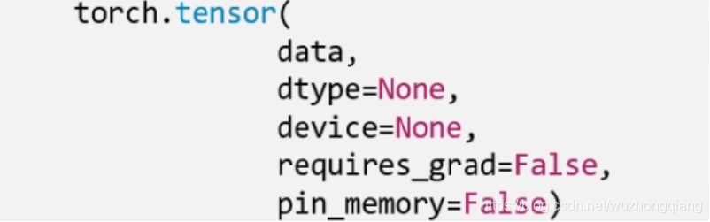
- data,就是我们的数据,可以是 list,也可以是 numpy。
- dtype 这个是指明数据类型, 默认与 data 的一致。
- device 是指明所在的设备
- requires_grad 是是否需要梯度, 在搭建神经网络的时候需要求导的那些参数这里要设置为 true。
- pin_memory 是否存于锁页内存,这个设置为 False 就可以。
下面就具体代码演示:
arr = np.ones((3, 3))print('ndarry的数据类型:', arr.dtype)t = torch.tensor(arr, device='cuda')print(t)ndarry的数据类型: float64tensor([[1., 1., 1.],[1., 1., 1.],[1., 1., 1.]], device='cuda:0', dtype=torch.float64)
通过 numpy 数组创建
torch.from_numpy(ndarry): 从 numpy 创建 tensor
注意:这个创建的 Tensor 与原 ndarray共享内存, 当修改其中一个数据的时候,另一个也会被改动。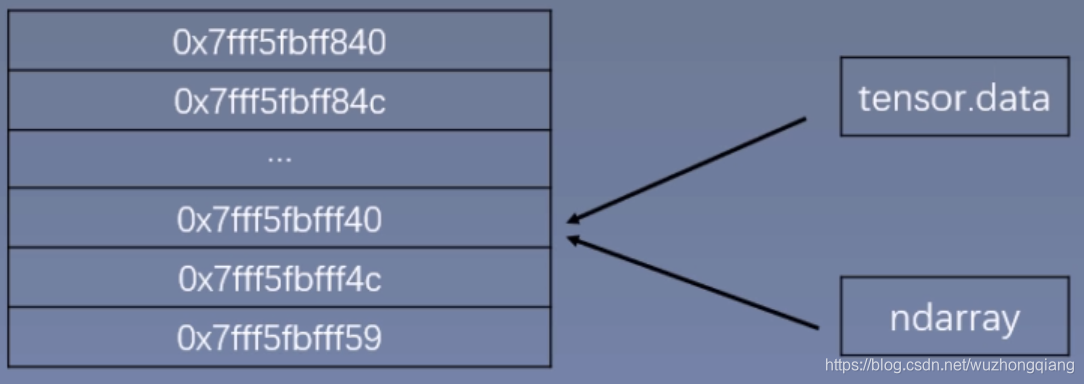
下面具体看代码演示(共享内存):
arr = np.array([[1, 2, 3], [4, 5, 6]])t = torch.from_numpy(arr)print(arr, '\n',t)arr[0, 0] = 0print('*' * 10)print(arr, '\n',t)t[1, 1] = 100print('*' * 10)print(arr, '\n',t)[[1 2 3][4 5 6]]tensor([[1, 2, 3],[4, 5, 6]], dtype=torch.int32)**********[[0 2 3][4 5 6]]tensor([[0, 2, 3],[4, 5, 6]], dtype=torch.int32)**********[[ 0 2 3][ 4 100 6]]tensor([[ 0, 2, 3],[ 4, 100, 6]], dtype=torch.int32)
依据数值创建
- torch.zeros(): 依 size 创建全 0 的张量
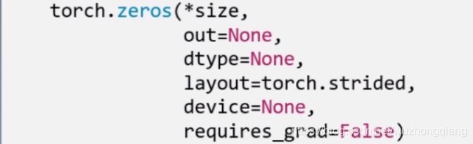
- layout 这个是内存中的布局形式, 一般采用默认就可以。
- out,表示输出张量,就是再把这个张量赋值给别的一个张量,但是这两个张量是一样的,指的同一个内存地址。看代码:```python out_t = torch.tensor([1]) t = torch.zeros((3, 3), out=out_t)
print(out_t, ‘\n’, t) print(id(t), id(out_t), id(t) == id(out_t))
tensor([[0, 0, 0], [0, 0, 0], [0, 0, 0]]) tensor([[0, 0, 0], [0, 0, 0], [0, 0, 0]]) 2575719258696 2575719258696 True
- torch.zeros_like(input, dtype=None, layout=None, device=None, requires_grad=False) : 这个是创建与 input 同**形状**的全 0 张量```pythont = torch.zeros_like(out_t)print(t)tensor([[0, 0, 0],[0, 0, 0],[0, 0, 0]])
- 除了全 0 张量, 还可以创建全 1 张量, 用法和上面一样,torch.ones(), torch.ones_like(), 还可以自定义数值张量:torch.full(), torch.full_like()
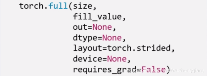
这里的 fill_value 就是要填充的值。
t = torch.full((3,3), 10)tensor([[10., 10., 10.],[10., 10., 10.],[10., 10., 10.]])
- torch.arange(): 创建等差的 1 维张量,数值区间[start, end), 注意这是右边开,取不到最后的那个数。
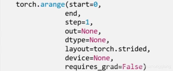
这个和 numpy 的差不多,这里的 step 表示的步长。
t = torch.arange(2, 10, 2)
- torch.linspace(): 创建均分的 1 维张量, 数值区间[start, end] 注意这里都是闭区间,和上面的区分。
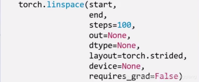
这里是右闭, 能取到最后的值,并且这里的 steps 是数列的长度而不是步长。
t = torch.linspace(2, 10, 5)t = torch.linspace(2, 10, 6)
除了创建均分数列,还可以创建对数均分数列: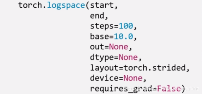
这里的 base 表示以什么为底。
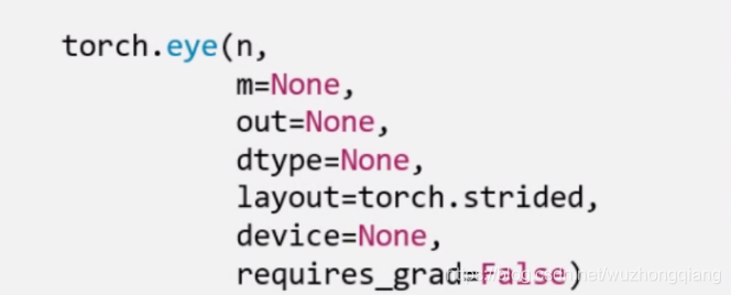
- torch.eye(): 创建单位对角矩阵, 默认是方阵
依概率分布创建张量
torch.normal(): 生成正态分布(高斯分布), 这个使用的比较多
mean 是均值,std 是标准差。 但是这个地方要注意, 根据 mean 和 std,分别各有两种取值,所以这里会有四种模式:
- mean 为标量, std 为标量
- mean 为标量, std 为张量
- mean 为张量, std 为标量
- mean 为张量,std 为张量
这个看代码来的直接:
t_normal = torch.normal(0, 1, size=(4,))print(t_normal)std = torch.arange(1, 5, dtype=torch.float)print(std.dtype)t_normal2 = torch.normal(1, std)print(t_normal2)mean = torch.arange(1, 5, dtype=torch.float)t_normal3 = torch.normal(mean, 1)print(t_normal3)mean = torch.arange(1, 5, dtype=torch.float)std = torch.arange(1, 5, dtype=torch.float)t_normal4 = torch.normal(mean, std)print(t_normal4)
下面一个是标准正态分布:torch.randn(), torch.randn_like()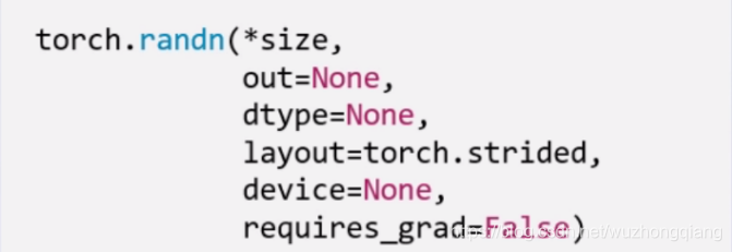
生成均匀分布:torch.rand(), rand_like() 在[0,1) 生成均匀分布
torch.randint(), torch.randint_like(): 区间[low,hight) 生成整数均匀分布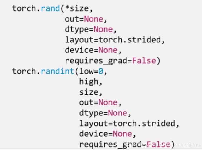
下面看最后两个:
torch.randperm(n): 生成从 0 - n-1 的随机排列, n 是张量的长度, 经常用来生成一个乱序索引。
torch.bernoulli(input): 以 input 为概率,生成伯努利分布 (0-1 分布,两点分布), input: 概率值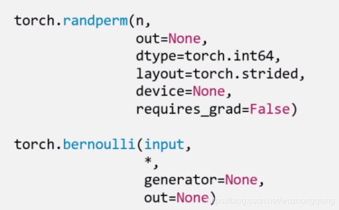
张量的操作
这次整理张量的基本操作,比如张量的拼接,切分,索引和变换以及数学运算等,并基于所学习的知识,实现线性回归模型。
张量的基本操作
1. 张量的拼接
- torch.cat(tensors, dim=0, out=None): 将张量按维度 dim 进行拼接, tensors 表示张量序列, dim 要拼接的维度
- torch.stack(tensors, dim=0, out=None): 在新创建的维度 dim 上进行拼接, tensors 表示张量序列, dim 要拼接的维度
stack 会新创建一个维度,然后完成拼接。还是看代码:
t = torch.ones((2, 3))print(t)t_0 = torch.cat([t, t], dim=0)t_1 = torch.cat([t, t], dim=1)print(t_0, t_0.shape)print(t_1, t_1.shape)tensor([[1., 1., 1.],[1., 1., 1.]])tensor([[1., 1., 1.],[1., 1., 1.],[1., 1., 1.],[1., 1., 1.]]) torch.Size([4, 3])tensor([[1., 1., 1., 1., 1., 1.],[1., 1., 1., 1., 1., 1.]]) torch.Size([2, 6])
cat 是在原来的基础上根据行和列,进行拼接, 我发现一个问题,就是浮点数类型拼接才可以,long 类型拼接会报错。
下面我们看看stack 方法:
t_stack = torch.stack([t,t,t], dim=0)print(t_stack)print(t_stack.shape)t_stack1 = torch.stack([t, t, t], dim=1)print(t_stack1)print(t_stack1.shape)tensor([[[1., 1., 1.],[1., 1., 1.]],[[1., 1., 1.],[1., 1., 1.]],[[1., 1., 1.],[1., 1., 1.]]])torch.Size([3, 2, 3])tensor([[[1., 1., 1.],[1., 1., 1.],[1., 1., 1.]],[[1., 1., 1.],[1., 1., 1.],[1., 1., 1.]]])torch.Size([2, 3, 3])
stack 是根据给定的维度新增了一个新的维度,在这个新维度上进行拼接, 这个. stack 与其说是从新维度上拼接,不太好理解,其实是新加了一个维度 Z 轴,只不过 dim=0 和 dim=1 的视角不同罢了。 dim=0 的时候,是横向看,dim=1 是纵向看。
所以这两个使用的时候要小心,看好了究竟是在原来的维度上拼接到一块,还是从新维度上拼接到一块。
2. 张量的切分
torch.chunk(input, chunks, dim=0): 将张量按维度 dim 进行平均切分, 返回值是张量列表,注意,如果不能整除, 最后一份张量小于其他张量。 chunks 代表要切分成几份。 下面看一下代码实现:
a = torch.ones((2, 7))list_of_tensors = torch.chunk(a, dim=1, chunks=3)print(list_of_tensors)for idx, t in enumerate(list_of_tensors):print("第{}个张量:{}, shape is {}".format(idx+1, t, t.shape))(tensor([[1., 1., 1.],[1., 1., 1.]]), tensor([[1., 1., 1.],[1., 1., 1.]]), tensor([[1.],[1.]]))第1个张量:tensor([[1., 1., 1.],[1., 1., 1.]]), shape is torch.Size([2, 3])第2个张量:tensor([[1., 1., 1.],[1., 1., 1.]]), shape is torch.Size([2, 3])第3个张量:tensor([[1.],[1.]]), shape is torch.Size([2, 1])
torch.split(tensor, split_size_or_sections, dim=0): 这个也是将张量按维度 dim 切分,但是这个更加强大, 可以指定切分的长度, split_size_or_sections 为 int 时表示每一份的长度, 为 list 时,按 list 元素切分```
t = torch.ones((2, 5))
list_of_tensors = torch.split(t, [2, 1, 2], dim=1)
for idx, t in enumerate(list_of_tensors):
print(“第{}个张量:{}, shape is {}”.format(idx+1, t, t.shape))
第1个张量:tensor([[1., 1.], [1., 1.]]), shape is torch.Size([2, 2]) 第2个张量:tensor([[1.], [1.]]), shape is torch.Size([2, 1]) 第3个张量:tensor([[1., 1.], [1., 1.]]), shape is torch.Size([2, 2])
<br />所以切分,也有两个函数,.chunk 和. split。- .chunk 切分的规则就是提供张量,切分的维度和几份, 比如三份, 先计算每一份的大小,也就是这个维度的长度除以三,然后上取整,就开始沿着这个维度切,最后不够一份大小的,也就那样了。 所以长度为 7 的这个维度,3 块,每块 7/3 上取整是 3, 然后第一块 3,第二块是 3,第三块 1。这样切- .split 这个函数的功能更加强大,它可以指定每一份的长度,只要传入一个列表即可,或者也有一个整数,表示每一份的长度,这个就根据每一份的长度先切着, 看看能切几块算几块。 不过列表的那个好使,可以自己指定每一块的长度,但是注意一下,这个长度的总和必须是维度的那个总长度才用办法切。<a name="oBbCY"></a>#### 3. 张量的索引torch.index_select(input, dim, index, out=None): 在维度 dim 上,按 index 索引数据,返回值,以 index 索引数据拼接的张量。```jsont = torch.randint(0, 9, size=(3, 3))print(t)idx = torch.tensor([0, 2], dtype=torch.long)t_select = torch.index_select(t, dim=1, index=idx)print(t_select)tensor([[3, 7, 3],[4, 3, 7],[5, 8, 0]])tensor([[3, 3],[4, 7],[5, 0]])
torch.masked_select(input, mask, out=None): 按 mask 中的 True 进行索引,返回值:一维张量。 input 表示要索引的张量, mask 表示与 input 同形状或者可以广播的布尔类型的张量。 这种情况在选择符合某些特定条件的元素的时候非常好使, 注意这个是返回一维的张量。下面看代码:```
mask = t.ge(5)
print(“mask: \n”, mask)
t_select1 = torch.masked_select(t, mask)
print(t_select1)
mask: tensor([[False, True, False], [False, False, True], [ True, True, False]]) tensor([7, 7, 5, 8])
<br />所以张量的索引,有两种方式:.index_select 和. masked_select- .index_select: 按照索引查找 需要先指定一个 Tensor 的索引量,然后指定类型是 long 的- .masked_select: 就是按照值的条件进行查找,需要先指定条件作为 mask<a name="czIgD"></a>#### 4. 张量的变换torch.reshape(input, shape): 变换张量的形状,这个很常用, input 表示要变换的张量,shape 表示新张量的形状。 但注意,当张量在内存中是连续时, 新张量与 input 共享数据内存```jsont = torch.randperm(8)print(t)t_reshape = torch.reshape(t, (-1, 2, 2))print("t:{}\nt_reshape:\n{}".format(t, t_reshape))t[0] = 1024print("t:{}\nt_reshape:\n{}".format(t, t_reshape))print("t.data 内存地址:{}".format(id(t.data)))print("t_reshape.data 内存地址:{}".format(id(t_reshape.data)))tensor([2, 4, 3, 1, 5, 6, 7, 0])t:tensor([2, 4, 3, 1, 5, 6, 7, 0])t_reshape:tensor([[[2, 4],[3, 1]],[[5, 6],[7, 0]]])t:tensor([1024, 4, 3, 1, 5, 6, 7, 0])t_reshape:tensor([[[1024, 4],[ 3, 1]],[[ 5, 6],[ 7, 0]]])t.data 内存地址:1556953167336t_reshape.data 内存地址:1556953167336
上面这两个是共内存的, 一个改变另一个也会改变。这个要注意一下。
torch.transpose(input, dim0, dim1): 交换张量的两个维度, 矩阵的转置常用, 在图像的预处理中常用, dim表示要交换的维度```json
t = torch.rand((2, 3, 4))
print(t)
t_transpose = torch.transpose(t, dim0=0, dim1=2)
print(“t shape:{}\nt_transpose shape: {}”.format(t.shape, t_transpose.shape))
tensor([[[0.7480, 0.5601, 0.1674, 0.3333], [0.4648, 0.6332, 0.7692, 0.2147], [0.7815, 0.8644, 0.6052, 0.3650]],
[[0.2536, 0.1642, 0.2833, 0.3858],[0.8337, 0.6173, 0.3923, 0.1878],[0.8375, 0.2109, 0.4282, 0.4974]]])
t shape:torch.Size([2, 3, 4]) t_transpose shape: torch.Size([4, 3, 2]) tensor([[[0.7480, 0.2536], [0.4648, 0.8337], [0.7815, 0.8375]],
[[0.5601, 0.1642],[0.6332, 0.6173],[0.8644, 0.2109]],[[0.1674, 0.2833],[0.7692, 0.3923],[0.6052, 0.4282]],[[0.3333, 0.3858],[0.2147, 0.1878],[0.3650, 0.4974]]])
<br />torch.t(input): 2 维张量的转置, 对矩阵而言,相当于 torch.transpose(inpuot, 0,1)<br />torch.squeeze(input, dim=None, out=None): 压缩长度为 1 的维度, dim 若为 None,移除所有长度为 1 的轴,若指定维度,当且仅当该轴长度为 1 时可以被移除```jsont = torch.rand((1, 2, 3, 1))t_sq = torch.squeeze(t)t_0 = torch.squeeze(t, dim=0)t_1 = torch.squeeze(t, dim=1)print(t.shape)print(t_sq.shape)print(t_0.shape)print(t_1.shape)
torch.unsqueeze(input, dim, out=None): 依据 dim 扩展维度
张量的数学运算
标量运算
Pytorch 中提供了丰富的数学运算,可以分为三大类: 加减乘除, 对数指数幂函数,三角函数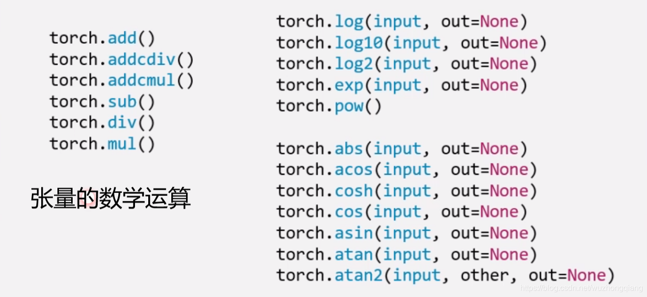
这里重点演示一下加法这个函数, 因为这个函数有一个小细节:
torch.add(input, alpha=1, other, out=None): 逐元素计算 input+alpha * other。 注意人家这里有个 alpha,叫做乘项因子。类似权重的个东西。
这个东西让计算变得更加简洁, 比如线性回归我们知道有个 y = wx + b, 在这里直接一行代码 torch.add(b, w, x) 就搞定。 类似的还有两个方法:
torch.addcdiv(input, value=1, tensor1, tensor2, out=None):
这个实现了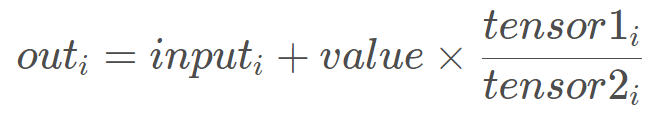
torch.addcmul(input, value=1, tensor1, tensor2, out=None)
这个实现了
这个在优化的时候经常会用到。
t_0 = torch.randn((3, 3))t_1 = torch.ones_like(t_0)t_add = torch.add(t_0, 10, t_1)print("t_0:\n{}\nt_1:\n{}\nt_add_10:\n{}".format(t_0, t_1, t_add))t_0:tensor([[-0.4133, 1.4492, -0.1619],[-0.4508, 1.2543, 0.2360],[ 1.0054, 1.2767, 0.9953]])t_1:tensor([[1., 1., 1.],[1., 1., 1.],[1., 1., 1.]])t_add_10:tensor([[ 9.5867, 11.4492, 9.8381],[ 9.5492, 11.2543, 10.2360],[11.0054, 11.2767, 10.9953]])
向量运算
向量运算符只在一个特定轴上运算,将一个向量映射到一个标量或者另外一个向量。
a = torch.arange(1,10).float()print(torch.sum(a))print(torch.mean(a))print(torch.max(a))print(torch.min(a))print(torch.prod(a))print(torch.std(a))print(torch.var(a))print(torch.median(a))
cum 累积
a = torch.arange(1,10)print(torch.cumsum(a,0))print(torch.cumprod(a,0))print(torch.cummax(a,0).values)print(torch.cummax(a,0).indices)print(torch.cummin(a,0))
张量排序
a = torch.tensor([[9,7,8],[1,3,2],[5,6,4]]).float()print(torch.topk(a,2,dim = 0),"\n")print(torch.topk(a,2,dim = 1),"\n")print(torch.sort(a,dim = 1),"\n")
矩阵运算
矩阵必须是二维的。类似 torch.tensor([1,2,3]) 这样的不是矩阵。
矩阵运算包括:矩阵乘法,矩阵转置,矩阵逆,矩阵求迹,矩阵范数,矩阵行列式,矩阵求特征值,矩阵分解等运算。
矩阵乘法
json
a = torch.tensor([[1,2],[3,4]])
b = torch.tensor([[2,0],[0,2]])
print(a@b)
转置
json
a = torch.tensor([[1.0,2],[3,4]])
print(a.t())
矩阵求逆
json
a = torch.tensor([[1.0,2],[3,4]])
print(torch.inverse(a))
矩阵求迹
json
a = torch.tensor([[1.0,2],[3,4]])
print(torch.trace(a))
求范数和行列式```json a = torch.tensor([[1.0,2],[3,4]]) print(torch.norm(a))
a = torch.tensor([[1.0,2],[3,4]]) print(torch.det(a))
6. 特征值和特征向量```jsona = torch.tensor([[1.0,2],[-5,4]],dtype = torch.float)print(torch.eig(a,eigenvectors=True))
QR 分解
json
a  = torch.tensor([[1.0,2.0],[3.0,4.0]])
q,r = torch.qr(a)
print(q,"\n")
print(r,"\n")
print(q@r)
SVD 分解```json a=torch.tensor([[1.0,2.0],[3.0,4.0],[5.0,6.0]])
u,s,v = torch.svd(a)
print(u,”\n”) print(s,”\n”) print(v,”\n”)
print(u@torch.diag(s)@v.t())
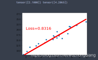
<a name="661f60dc"></a>## 搭建一个线性回归模型线性回归是分析一个变量与另外一 (多) 个变量之间关系的方法。 因变量是 y, 自变量是 x, 关系线性: <br />y = wx + b<br />任务就是求解 w,b。<br />我们的求解步骤:1. 确定模型: Model -> y = wx + b1. 选择损失函数: 这里用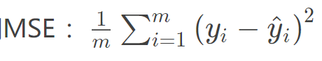3. 求解梯度并更新 w, b<br />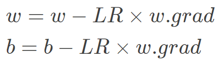<br />这就是我上面说的叫做代码逻辑的一种思路, 写代码往往习惯先有一个这样的一种思路,然后再去写代码的时候,就比较容易了。 而如果不系统的学一遍 Pytorch, 一上来直接上那种复杂的 CNN, LSTM 这种,往往这些代码逻辑不好形成,因为好多细节我们根本就不知道。 所以这次学习先从最简单的线性回归开始,然后慢慢的到复杂的那种网络。下面我们开始写一个线性回归模型:```jsonx = torch.rand(20, 1) * 10y = 2 * x + (5 + torch.randn(20, 1))w = torch.randn((1), requires_grad=True)b = torch.zeros((1), requires_grad=True)for iteration in range(100):wx = torch.mul(w, x)y_pred = torch.add(wx, b)loss = (0.5 * (y-y_pred)**2).mean()loss.backward()b.data.sub_(lr * b.grad)w.data.sub_(lr * w.grad)w.grad.data.zero_()b.grad.data.zero_()print(w.data, b.data)
我们看一下结果:
5. 总结
今天的学习内容结束, 下面简单的梳理一遍,其实小东西还是挺多的, 首先我们从 Pytorch 最基本的数据结构开始,认识了张量到底是个什么东西,说白了就是个多维数组,然后张量本身有很多的属性, 有关于数据本身的 data, dtype, shape, dtype, 也有关于求导的 requires_grad, grad, grad_fn, is_leaf。 然后学习了张量的创建方法, 比如直接创建,从数组创建,数值创建,按照概率创建等。 这里面涉及到了很多的创建函数 tensor(), from_numpy(), ones(), zeros(), eye(), full(), arange(), linspace(), normal(), randn(), rand(), randint(), randperm() 等等吧。
接着就是张量的操作部分, 有基本操作和数学运算, 基本操作部分有张量的拼接两个函数 (.cat, .stack), 张量的切分两个函数 (.chunk, .split), 张量的转置 (.reshape, .transpose, .t), 张量的索引两个函数 (.index_select, .masked_select)。 数学运算部分,也是很多数学函数,有加减乘除的,指数底数幂函数的,三角函数的很多。
最后基于上面的所学完成了一个简单的线性回归。 下面以一张思维导图把这一篇文章的内容拎起来: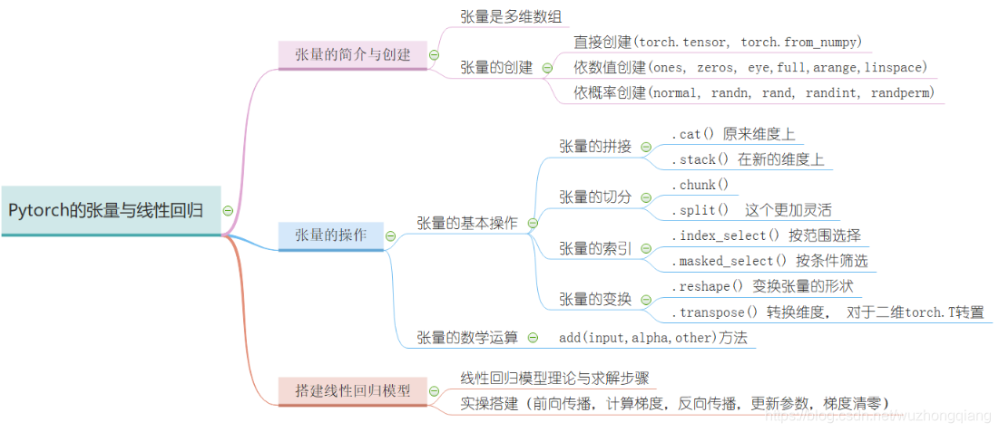

若有收获,就点个赞吧
0 人点赞
