Bounding Box Regression

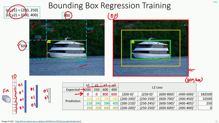
Typically, regression models are applied to problems such as:

• Predicting the price of a home
• Forecasting the stock market
• Determining the rate of a disease spreading through a population

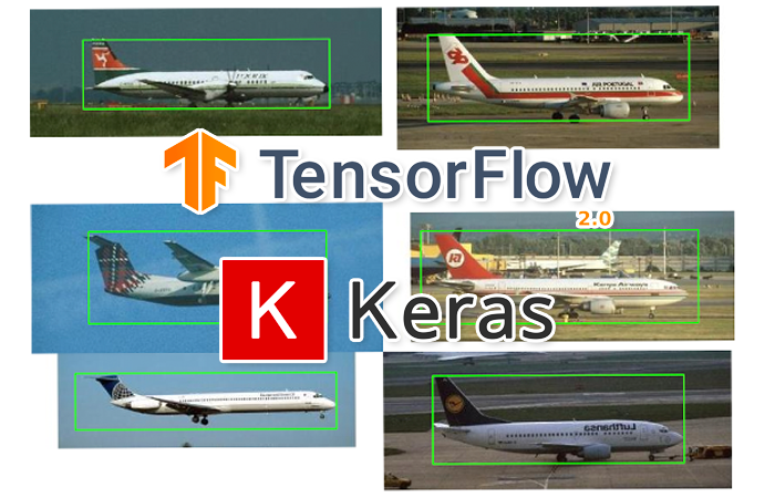
Multi-class Object Detection

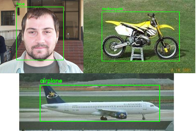
In order to create a multi-class object detector from scratch with Keras and TensorFlow, we’ll need to modify the network head of our architecture. The order of operations will be to:

1. Take VGG16 (pre-trained on ImageNet) and remove the fully-connected (FC) layer head
2. Construct a new FC layer head with two branches:
   1. Branch #1: A series of FC layers that end with a layer with
      1. four neurons, corresponding to the top-left and bottom-right (x, y)-coordinates of the predicted bounding box
      2. a sigmoid activation function, such that the output of each four neurons lies in the range [0, 1]. This branch is responsible for bounding box predictions.
   2. Branch #2: Another series of FC layers, but this one with a softmax classifier at the end. This branch is in charge of making class label predictions.
3. Place the new FC layer head (with the two branches) on top of the VGG16 body
4. Fine-tune the entire network for end-to-end object detection

Histogram of Oriented Gradients

Algorithms:

1. Sample P positive samples from your training data of the object(s) you want to detect and extract HOG descriptors from these samples.
2. Sample N negative samples from a negative training set that does not contain any of the objects you want to detect and extract HOG descriptors from these samples as well. In practice N >> P.
3. Train a Linear Support Vector Machine on your positive and negative samples.
4. Apply hard-negative mining. For each image and each possible scale of each image in your negative training set, apply the sliding window technique and slide your window across the image.
5. Take the false-positive samples found during the hard-negative mining stage, sort them by their confidence (i.e. probability) and re-train your classifier using these hard-negative samples.
6. Your classifier is now trained and can be applied to your test dataset. Again, just like in Step 4, for each image in your test set, and for each scale of the image, apply the sliding window technique. At each window extract HOG descriptors and apply your classifier.

Adversarial Images and Attacks

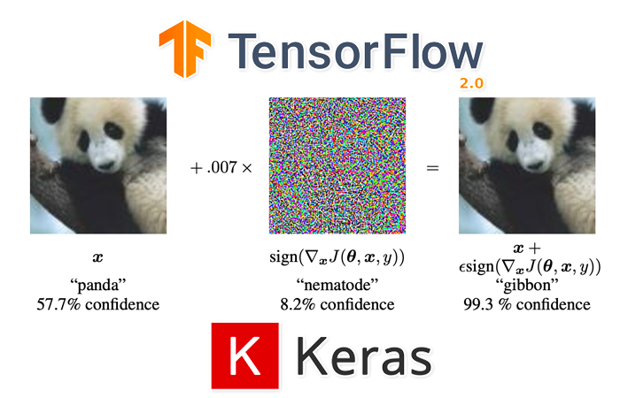
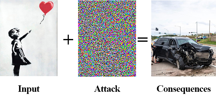
Adversarial attacks embed a message in an input image — but instead of a plaintext message meant for human consumption, an adversarial attack instead embeds a noise vector in the input image. This noise vector is purposely constructed to fool and confuse deep learning models.

Distance from Camera

triangle similarity:

• W - the width of a marker or object.
• D - the distance from camera to placed marker.
• P - the apparent width of the object taken by the camera.
• Derive the perceived focal length F of the camera:

as moving the camera both closer or farther away from the object/marker:

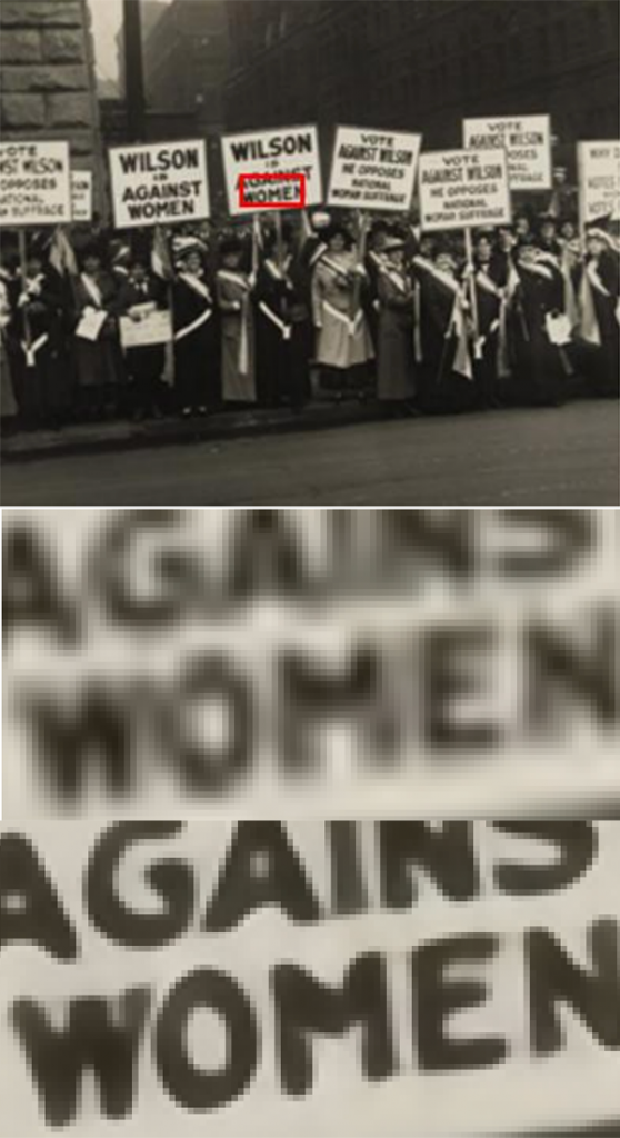
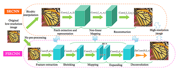
Super Resolution

GANs

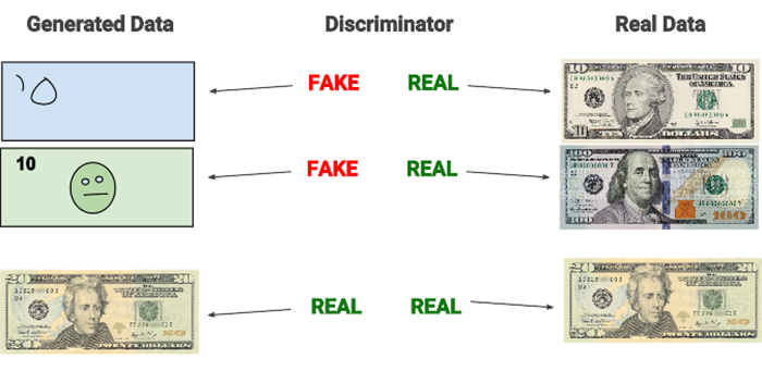
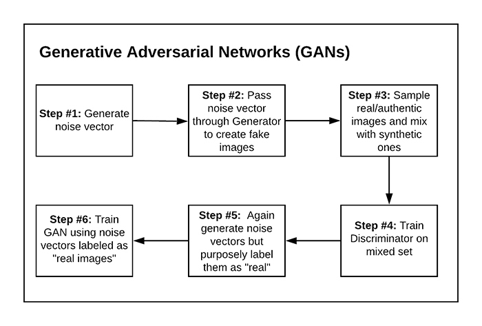
In order to generate synthetic images, we make use of two neural networks during training:

• A generator that accepts an input vector of randomly generated noise and produces an output “imitation” image that looks similar, if not identical, to the authentic image
• A discriminator or adversary that attempts to determine if a given image is an “authentic” or “fake”