- Bubble sheet scanner & test grader
- OMR
- Document Scanner
- Contour Sorting
- Perspective Transforms
- Binarization
- Contour Extraction
- Grading
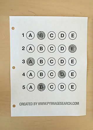
- More test results
- Shortcomings
- What’s More
- Source Code
- !/usr/bin/env python
- encoding: utf-8
- import the necessary packages
- construct the argument parse and parse the arguments
- define the answer key which maps the question number to the correct answer
- load the image, convert it to grayscale, blur it slightly, then find edges
- find contours in the edge map,
- then initialize the contour that corresponds to the document
- ensure that at least one contour was found
- apply a four point perspective transform to both
- the original image and grayscale image to obtain a top-down birds eye view of the paper
- apply Otsu’s thresholding method to binarize the warped
- piece of paper
- find contours in the thresholded image,
- then initialize the list of contours that correspond to questions
- loop over the contours
- sort the question contoudrs top-to-bottom,
- then initialize the total number of correct answers
- each question has 5 possible answers,
- to loop over the question in batches of 5
- grab the test taker
- cv2.imshow(“Original”, image)
One of my favorite parts of tutoring is demonstrating how to build actual solutions to problems using computer vision. Demonstrate how to implement a bubble sheet test scanner and grader using strictly computer vision and image processing techniques, along with the OpenCV library.
Bubble sheet scanner & test grader
The 7 steps to build a bubble sheet scanner and grader using Python and OpenCV. To accomplish this, our implementation will need to satisfy the following 7 steps:
- Step #1: Detect the exam in an image.
- Step #2: Apply a perspective transform to extract the top-down, birds-eye-view of the exam.
- Step #3: Extract the set of bubbles (i.e., the possible answer choices) from the perspective transformed exam.
- Step #4: Sort the questions/bubbles into rows.
- Step #5: Determine the marked (i.e., “bubbled in”) answer for each row.
- Step #6: Lookup the correct answer in our answer key to determine if the user was correct in their choice.
- Step #7: Repeat for all questions in the exam.
OMR
Optical Mark Recognition, or OMR for short, is the process of automatically analyzing human-marked documents and interpreting their results.
With the basic understanding of OMR, let’s build a computer vision system using Python and OpenCV that can read and grade bubble sheet tests.
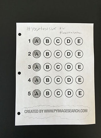
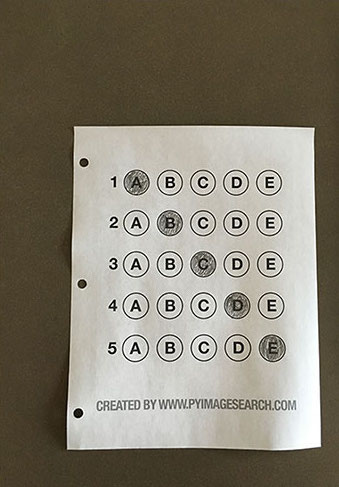
Below is an example filled in bubble sheet exam that I have put together for this project: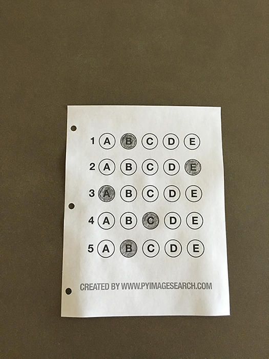
Document Scanner
Get started
#!/usr/bin/env python# encoding: utf-8# import the necessary packagesfrom imutils.perspective import four_point_transformfrom imutils import contoursimport numpy as npimport argparseimport imutilsimport cv2# construct the argument parse and parse the argumentsap = argparse.ArgumentParser()ap.add_argument("-i", "--image", required=False, default='omr_test_01.png', help="path to the input image")args = vars(ap.parse_args())# define the answer key which maps the question number# to the correct answerANSWER_KEY = {0: 1, 1: 4, 2: 0, 3: 3, 4: 1}
- Lines 4-10 import our required Python packages.
- Lines 14-15 parse our command line arguments. We only need a single switch here, —image , which is the path to the input bubble sheet test image that we are going to grade for correctness.
- Line 19 then defines our ANSWER_KEY .
As the name of the variable suggests, the ANSWER_KEY provides integer mappings of the question numbers to the index of the correct bubble.
In this case, a key of 0 indicates the first question, while a value of 1 signifies “B” as the correct answer (since “B” is the index 1 in the string “ABCDE”). As a second example, consider a key of 1 that maps to a value of 4 — this would indicate that the answer to the second question is “E”.
Preprocess input image
# load the image, convert it to grayscale, blur it slightly, then find edgesimage = cv2.imread(args["image"])gray = cv2.cvtColor(image, cv2.COLOR_BGR2GRAY)blurred = cv2.GaussianBlur(gray, (5, 5), 0)edged = cv2.Canny(blurred, 75, 200)
- Line 2 load our image from disk,
- Line 3 converting it to grayscale,
- Line 4 blurring it to reduce high frequency noise.
- Line 5 apply the Canny edge detector on to find the edges/outlines of the exam.
Below I have included a screenshot of our exam after applying edge detection: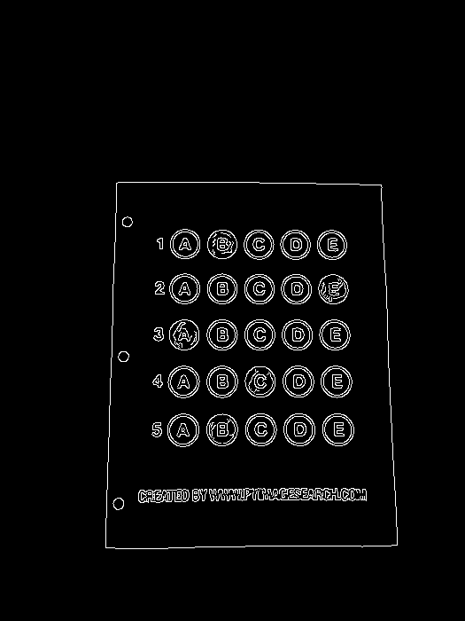
Notice how the edges of the document are clearly defined, with all four vertices of the exam being present in the image.
Contour Sorting
Obtaining this silhouette of the document is extremely important in our next step as we will use it as a marker to apply a perspective transform to the exam, obtaining a top-down, birds-eye-view of the document.
# find contours in the edge map, then initialize the contour that corresponds to the documentcnts = cv2.findContours(edged.copy(), cv2.RETR_EXTERNAL, cv2.CHAIN_APPROX_SIMPLE)cnts = imutils.grab_contours(cnts)docCnt = None# ensure that at least one contour was foundif len(cnts) > 0:# sort the contours according to their size in# descending ordercnts = sorted(cnts, key=cv2.contourArea, reverse=True)# loop over the sorted contoursfor c in cnts:# approximate the contourperi = cv2.arcLength(c, True)approx = cv2.approxPolyDP(c, 0.02 * peri, True)# if our approximated contour has four points,# then we can assume we have found the paperif len(approx) == 4:docCnt = approxbreakpasspass
- Line 7 making sure at least one contour was found on
- Line 10 sort our contours by their area (from largest to smallest). This implies that larger contours will be placed at the front of the list, while smaller contours will appear farther back in the list.
- Line 12 loop over each of our (sorted) contours. For each of them, approximate the contour, which in essence means we simplify the number of points in the contour, making it a “more basic” geometric shape.
- Line 18 make a check to see if our approximated contour has four points, and if it does, we assume that we have found the exam.
Now that we have the outline of our exam, we apply the cv2.findContours function to find the lines that correspond to the exam itself.
Below I have included an example image that demonstrates the docCnt variable being drawn on the original image: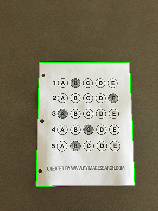
Sure enough, this area corresponds to the outline of the exam.
Perspective Transforms
Now that we have used contours to find the outline of the exam, we can apply a perspective transform to obtain a top-down, birds-eye-view of the document.
# apply a four point perspective transform to both the original image and grayscale image to obtain a top-down birds eye view of the paperpaper = four_point_transform(image, docCnt.reshape(4, 2))warped = four_point_transform(gray, docCnt.reshape(4, 2))
- Orders the (x, y)-coordinates of our contours in a specific, reproducible manner.
- Applies a perspective transform to the region.
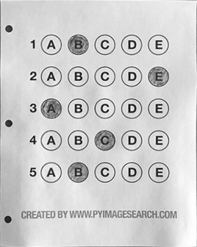
this function handles taking the “skewed” exam and transforms it, returning a top-down view of the document (original on the left, grayscale on the right):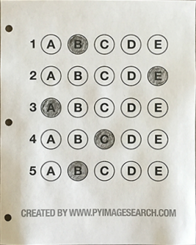
Binarization
The process of thresholding/segmenting the foreground from the background of the image:
# apply Otsu's thresholding method to binarize the warped piece of paperthresh = cv2.threshold(warped, 0, 255, cv2.THRESH_BINARY_INV | cv2.THRESH_OTSU)[1]
After applying Otsu’s thresholding method, our exam is now a binary image: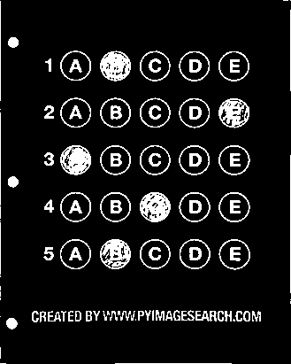
Notice how the background of the image is black, while the foreground is white.
Contour Extraction
the above binarization will allow us to once again apply contour extraction techniques to find each of the bubbles in the exam.
# find contours in the thresholded image,# then initialize the list of contours that correspond to questionscnts = cv2.findContours(thresh.copy(), cv2.RETR_EXTERNAL, cv2.CHAIN_APPROX_SIMPLE)cnts = imutils.grab_contours(cnts)questionCnts = []# loop over the contoursfor c in cnts:# compute the bounding box of the contour,# then use the bounding box to derive the aspect ratio(x, y, w, h) = cv2.boundingRect(c)ar = w / float(h)# in order to label the contour as a question,# region should be sufficiently wide, sufficiently tall,# and have an aspect ratio approximately equal to 1if w >= 20 and h >= 20 and ar >= 0.9 and ar <= 1.1:questionCnts.append(c)pass
- Lines 3-5 finding contours on our
threshbinary image, followed by initializing questionCnts , a list of contours that correspond to the questions/bubbles on the exam. - Line 8 loop over each of the individual contours to determine which regions of the image are bubbles.
- Line 11 compute the bounding box for each of these contours.
- Line 12 compute the aspect ratio, or more simply, the ratio of the width to the height.
In order for a contour area to be considered a bubble, the region should:
- Be sufficiently wide and tall (in this case, at least 20 pixels in both dimensions).
- Have an aspect ratio that is approximately equal to 1.
As long as these checks hold, we can update our questionCnts list and mark the region as a bubble. Below I have included a screenshot that has drawn the output of questionCnts on our image: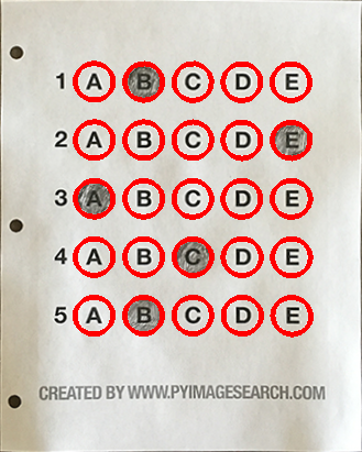
Notice how only the question regions of the exam are highlighted and nothing else.
Grading
We can now move on to the “grading” portion of our OMR system.
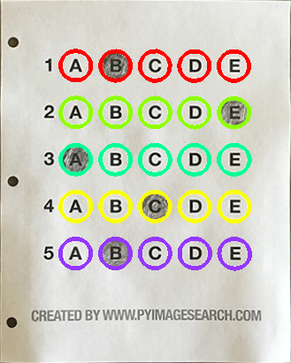
Each Row
# sort the question contours top-to-bottom,# then initialize the total number of correct answersquestionCnts = contours.sort_contours(questionCnts, method="top-to-bottom")[0]correct = 0# each question has 5 possible answers,# to loop over the question in batches of 5for (q, i) in enumerate(np.arange(0, len(questionCnts), 5)):# sort the contours for the current question from left to right,# then initialize the index of the bubbled answercnts = contours.sort_contours(questionCnts[i:i + 5])[0]bubbled = None
- Line 8 start looping over our questions. Since each question has 5 possible answers, we’ll apply NumPy array slicing and contour sorting to to sort the current set of contours from left to right.
- Line 11 ensures each row of contours are sorted into rows, from left-to-right.
Filled in Bubbles
To determine which bubble is filled in. we using our thresh image and counting the number of non-zero pixels (i.e., foreground pixels) in each bubble region.
# loop over the sorted contoursfor (j, c) in enumerate(cnts):# construct a mask that reveals only the current "bubble" for the questionmask = np.zeros(thresh.shape, dtype="uint8")cv2.drawContours(mask, [c], -1, 255, -1)# apply the mask to the thresholded image,# then count the number of non-zero pixels in the bubble areamask = cv2.bitwise_and(thresh, thresh, mask=mask)total = cv2.countNonZero(mask)# if the current total has a larger number of total non-zero pixels,# then we are examining the currently bubbled-in answerif bubbled is None or total > bubbled[0]:bubbled = (total, j)pass
- Line 2 handles looping over each of the sorted bubbles in the row.
- Line 4 We then construct a mask for the current bubble on.
- Lines 8-9 then count the number of non-zero pixels in the masked region.
- Line 12- 13 The more non-zero pixels we count, then the more foreground pixels there are, and therefore the bubble with the maximum non-zero count is the index of the bubble that the the test taker has bubbled in.
Clearly, the bubble associated with “B” has the most thresholded pixels, and is therefore the bubble that the user has marked on their exam.
Look up the correct answer
This next code block handles looking up the correct answer in the ANSWER_KEY, updating any relevant bookkeeper variables, and finally drawing the marked bubble on our image.
# initialize the contour color and the index of the *correct* answercolor = (0, 0, 255)k = ANSWER_KEY[q]# check to see if the bubbled answer is correctif k == bubbled[1]:color = (0, 255, 0)correct += 1# draw the outline of the correct answer on the testcv2.drawContours(paper, [cnts[k]], -1, color, 3)
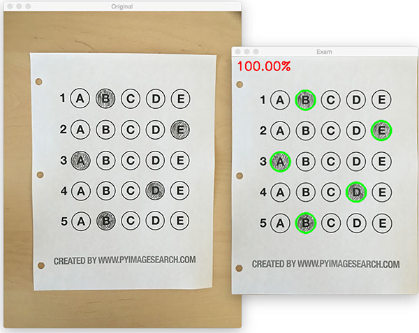
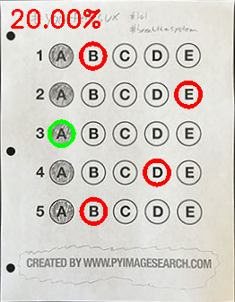
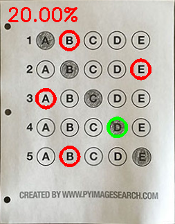
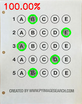
Based on whether the test taker was correct or incorrect yields which color is drawn on the exam. If the test taker is correct, we’ll highlight their answer in green. However, if the test taker made a mistake and marked an incorrect answer, we’ll let them know by highlighting the correct answer in red: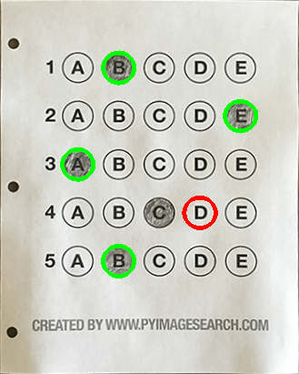
Give the grade
Our last code block handles scoring the exam and displaying the results to our screen.
# grab the test takerscore = (correct / 5.0) * 100print("[INFO] score: {:.2f}%".format(score))cv2.putText(paper, "{:.2f}%".format(score), (10, 30), cv2.FONT_HERSHEY_SIMPLEX, 0.9, (0, 0, 255), 2)cv2.imshow("Gader", paper)cv2.waitKey(0)
Below you can see the output of our fully graded example image: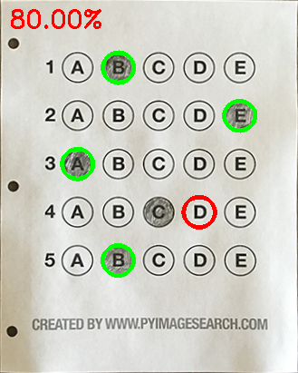
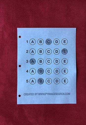
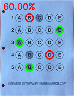
More test results
Shortcomings
Discuss some of the shortcomings of this current bubble sheet scanner system and how we can improve it in future iterations.
Why not circle detection?
Tuning the parameters to Hough circles on an image-to-image basis can be a real pain.
The real reason is: User error.
How many times, whether purposely or not, have you filled in outside the lines on your bubble sheet? I’m not expert, but I’d have to guess that at least 1 in every 20 marks a test taker fills in is “slightly” outside the lines.
The cv2.findContours function doesn’t care if the bubble is “round”, “perfectly round”, or “oh my god, what the hell is that?”.
What’s More
While I was able to get the barebones of a working bubble sheet test scanner implemented, there are certainly a few areas that need improvement. The most obvious area for improvement is the logic to handle non-filled in bubbles.
Since we determine if a particular bubble is “filled in” simply by counting the number of thresholded pixels in a row and then sorting in descending order, this can lead to two problems:
- What happens if a user does not bubble in an answer for a particular question?
- What if the user is nefarious and marks multiple bubbles as “correct” in the same row?
Not bubbled in a row
If a reader chooses not to bubble in an answer for a particular row, then we can place a minimum threshold when we computecv2.countNonZero.
Multi-bubbled in a row
Apply our thresholding and count step, this time keeping track if there are multiple bubbles that have atotalthat exceeds some pre-defined value. If so, we can invalidate the question and mark the question as incorrect.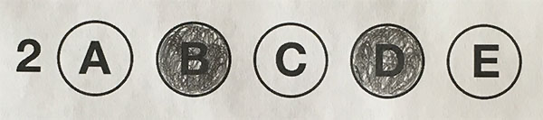
Source Code
the complete source code can be found bellow: ```python!/usr/bin/env python
encoding: utf-8
import the necessary packages
from imutils.perspective import four_point_transform from imutils import contours import numpy as np import argparse import imutils import cv2
construct the argument parse and parse the arguments
ap = argparse.ArgumentParser() ap.add_argument(“-i”, “—image”, required=False, default=’omr_test_01.png’, help=”path to the input image”) args = vars(ap.parse_args())
define the answer key which maps the question number to the correct answer
ANSWER_KEY = {0: 1, 1: 4, 2: 0, 3: 3, 4: 1}
load the image, convert it to grayscale, blur it slightly, then find edges
image = cv2.imread(args[“image”]) gray = cv2.cvtColor(image, cv2.COLOR_BGR2GRAY) blurred = cv2.GaussianBlur(gray, (5, 5), 0) edged = cv2.Canny(blurred, 75, 200)
cv2.imshow(‘edged’, edged) cv2.waitKey(0)
find contours in the edge map,
then initialize the contour that corresponds to the document
cnts = cv2.findContours(edged.copy(), cv2.RETR_EXTERNAL, cv2.CHAIN_APPROX_SIMPLE) cnts = imutils.grab_contours(cnts) docCnt = None
ensure that at least one contour was found
if len(cnts) > 0:
# sort the contours according to their size in descending ordercnts = sorted(cnts, key=cv2.contourArea, reverse=True)# loop over the sorted contoursfor c in cnts:# approximate the contourperi = cv2.arcLength(c, True)approx = cv2.approxPolyDP(c, 0.02 * peri, True)# if our approximated contour has four points,# then we can assume we have found the paperif len(approx) == 4:docCnt = approxbreakpass
if docCnt is not None: outline = image.copy() cv2.drawContours(outline, [docCnt], -1, (0, 255, 0), 2) cv2.imshow(“Outline”, outline) cv2.waitKey(0)
apply a four point perspective transform to both
the original image and grayscale image to obtain a top-down birds eye view of the paper
paper = four_point_transform(image, docCnt.reshape(4, 2)) warped = four_point_transform(gray, docCnt.reshape(4, 2))
cv2.imshow(“Original”, imutils.resize(paper, height = 500)) cv2.waitKey(0)
cv2.imshow(“Scanned”, imutils.resize(warped, height = 500)) cv2.waitKey(0)
apply Otsu’s thresholding method to binarize the warped
piece of paper
thresh = cv2.threshold(warped, 0, 255, cv2.THRESH_BINARY_INV | cv2.THRESH_OTSU)[1] cv2.imshow(“thresh”, thresh) cv2.waitKey(0)
find contours in the thresholded image,
then initialize the list of contours that correspond to questions
cnts = cv2.findContours(thresh.copy(), cv2.RETR_EXTERNAL, cv2.CHAIN_APPROX_SIMPLE) cnts = imutils.grab_contours(cnts) questionCnts = []
loop over the contours
for c in cnts:
# compute the bounding box of the contour,# then use the bounding box to derive the aspect ratio(x, y, w, h) = cv2.boundingRect(c)ar = w / float(h)# in order to label the contour as a question,# region should be sufficiently wide, sufficiently tall,# and have an aspect ratio approximately equal to 1if w >= 20 and h >= 20 and ar >= 0.9 and ar <= 1.1:questionCnts.append(c)pass
questions = paper.copy() for cnt in questionCnts: cv2.drawContours(questions, [cnt], -1, (0, 0, 255), 3) pass cv2.imshow(“questions”, questions) cv2.waitKey(0)
ques_rows = paper.copy() ques_colors = [(0, 0, 255), (0, 255, 142), (150, 255, 0), (0, 255, 251), (255, 55, 148)]
sort the question contoudrs top-to-bottom,
then initialize the total number of correct answers
questionCnts = contours.sort_contours(questionCnts, method=”top-to-bottom”)[0] correct = 0
each question has 5 possible answers,
to loop over the question in batches of 5
for (q, i) in enumerate(np.arange(0, len(questionCnts), 5)):
# sort the contours for the current question from left to right,# then initialize the index of the bubbled answercnts = contours.sort_contours(questionCnts[i:i + 5])[0]bubbled = Nonecv2.drawContours(ques_rows, cnts, -1, ques_colors[i//5], 3)# loop over the sorted contoursfor (j, c) in enumerate(cnts):# construct a mask that reveals only the current "bubble" for the questionmask = np.zeros(thresh.shape, dtype="uint8")cv2.drawContours(mask, [c], -1, 255, -1)# apply the mask to the thresholded image,# then count the number of non-zero pixels in the bubble areamask = cv2.bitwise_and(thresh, thresh, mask=mask)total = cv2.countNonZero(mask)# if the current total has a larger number of total non-zero pixels,# then we are examining the currently bubbled-in answerif bubbled is None or total > bubbled[0]:bubbled = (total, j)pass# initialize the contour color and the index of the *correct* answercolor = (0, 0, 255)k = ANSWER_KEY[q]# check to see if the bubbled answer is correctif k == bubbled[1]:color = (0, 255, 0)correct += 1# draw the outline of the correct answer on the testcv2.drawContours(paper, [cnts[k]], -1, color, 3)pass
cv2.imshow(“rows”, ques_rows) cv2.waitKey(0)
grab the test taker
score = (correct / 5.0) * 100 print(“[INFO] score: {:.2f}%”.format(score))
cv2.imshow(“Original”, image)
cv2.imshow(“Exam”, paper) cv2.waitKey(0)
cv2.putText(paper, “{:.2f}%”.format(score), (10, 30), cv2.FONT_HERSHEY_SIMPLEX, 0.9, (0, 0, 255), 2) cv2.imshow(“Gader”, paper) cv2.waitKey(0)
cv2.destroyAllWindows() ```

若有收获,就点个赞吧
0 人点赞
