概述
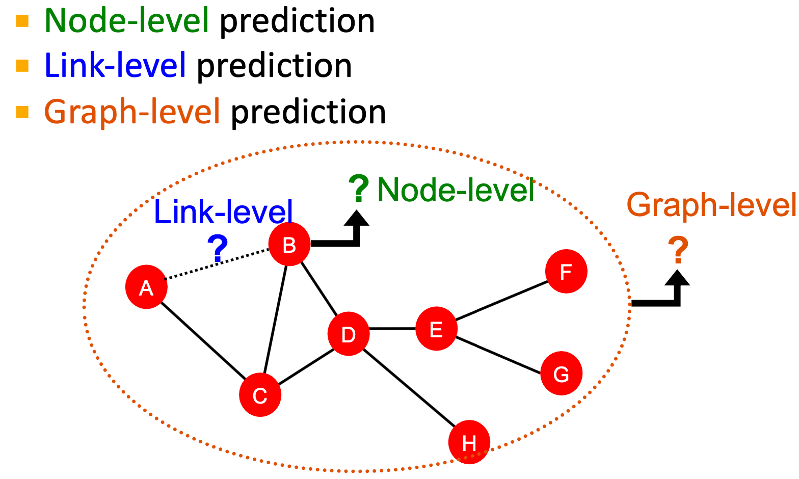
基于给定的一个新的node/link/graph,获得其特征,并做出预测。
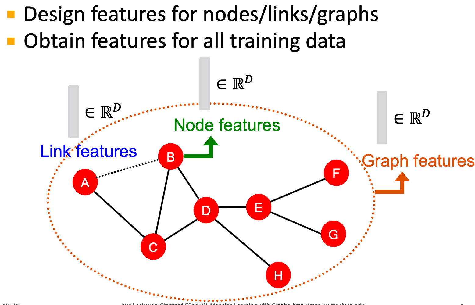
在图形上使用有效的特性是获得良好测试性能的关键。传统的ML pipeline使用手动设计的特征。本节概述以下预测任务的传统特征:
- Node-level prediction
- Link-level prediction
- Graph-level prediction
为了简单化,我们聚焦在无向图上。
图中的机器学习:给定 ,学习一个函数
 。
。
Node-level任务与特征
node-level特征的目标是:描述网络中节点的结构和位置,如节点度、节点中心性、聚类系数、graphlets等。
Node Features (Node Degree)
节点 的度
的度 是该节点拥有的边(相邻节点)的数量,平等地对待所有相邻节点。
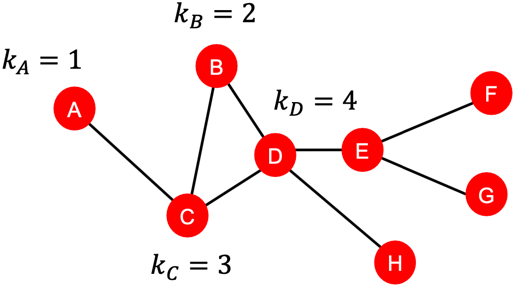
Node Features (Node Centrality)
节点度计算相邻节点,但不考虑它们的重要性。节点中心性(Node centrality) 考虑图中节点的重要性。
构建重要性模型的不同方法:
- Eigenvector centrality
- Betweenness centrality
- Closeness centrality
-
特征向量中心性 Eigenvector centrality
如果一个节点
 被重要的相邻节点
 所包围,那么这个节点就很重要。
我们将节点 的中心性定义为相邻节点的中心性之和:
 ,其中
,其中 是一正的常数。
上面的等式是以递归的方式对中心性进行的定时。我们怎么解它?
可将上式递归等式用矩阵形式表示: ,其中
,其中 表示邻接矩阵,
 ;
; 是中心性向量。
一个邻接矩阵 存在多对特征向量和特征值。中心性的值通常为正数,所以选择中心性需要考虑所有元素均为正数的特征向量。根据Perron- Frobenius定理,一个元素全为正的实方阵具有唯一的最大特征值,其对应的特征向量的元素全为正。因此可选择最大的特征值
 ,将它相应的特征向量作为中心性向量。
结论: 中心性是特征向量;
- 最大特征值
 总是正的,且唯一(通过Perron- Frobenius定理);
 -
介数中心性 Betweenness centrality
检查是否在图中处于重要位置。具体地,若许多路通过同一个节点,那么该节点处于图中的一个重要位置。节点
 的介数定义为:
紧密中心性 Closeness centrality
如果一个节点到其他所有节点的最短路径长度很小,那么这个节点就很重要。

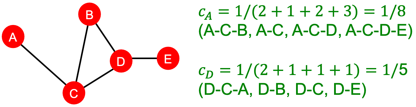
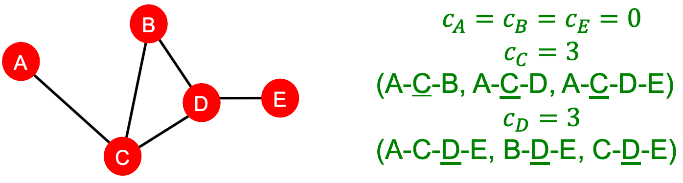
Node Features (Clustering Coefficient)
Node Features (Graphlets)
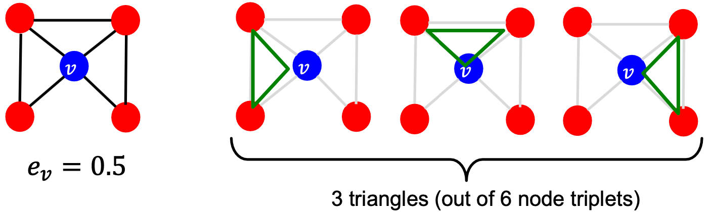
聚类系数计算自我网络中的三角形数
我们可以通过计算#(预先指定的子图,即graphlets)来一般化上面的内容。
Graphlets:有根连通非同构子图。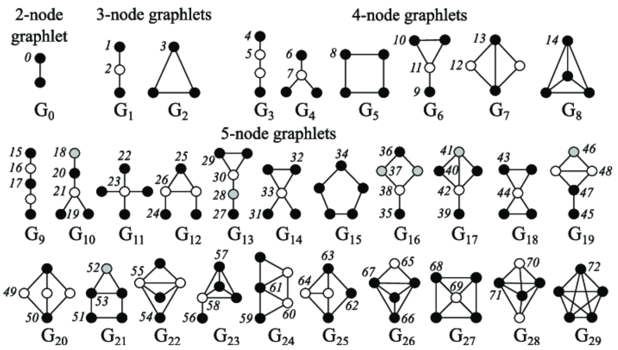
Graphlet度向量(GDV):节点的基于Graphlet的特性;
- 度:计算节点接触的边数
- 聚类系数:计数节点接触的三角形数
- GDV统计节点接触的#(graphlets)
 对应的特征向量
 ,用于中心性。
 的相邻节点的连接程度:
 表示#(节点
 的邻居节点)
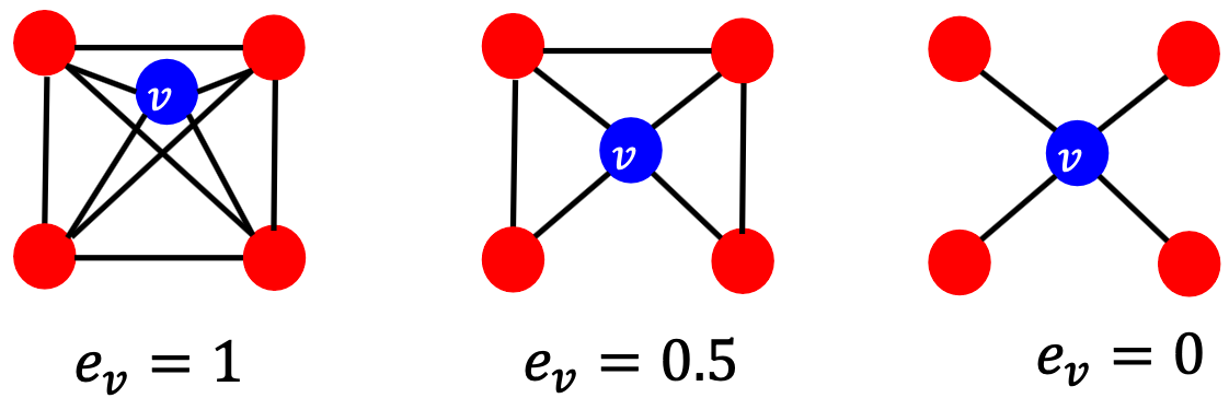
GDV:根在给定节点上的graphlets的计数向量。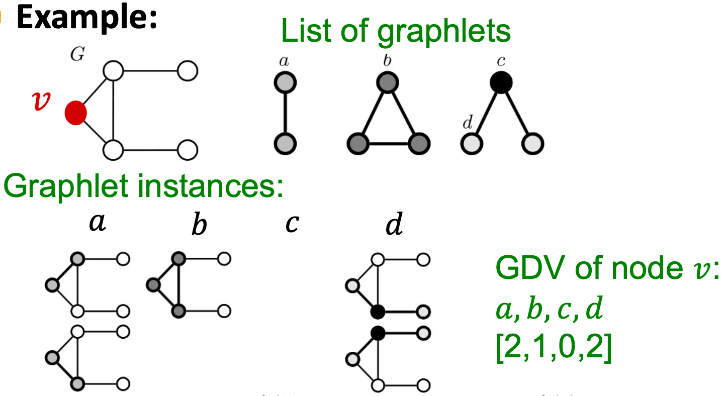
考虑2到5个节点上的graphlets,我们得到:
- 73坐标向量是一个节点的特征,描述了节点的邻居的拓扑结构;
- 在4跳的距离内捕捉到它的相互连接。
Graphlet度向量提供了节点本地网络拓扑的度量:
比较两个节点的向量提供了比节点度或聚类系数更详细的局部拓扑相似性度量。
Node-Level Feature (Summary)
我们已经介绍了获取节点特性的不同方法,可分分类为:
Importance-based features,捕获一个节点的重要性是在一个图中(用于预测图中有影响力的节点,如预测社交网络中的名人用户):
- Node degree,只是计算相邻节点的数量
- Different node centrality measures,在一个图中重要性邻近节点;不同的选择,如特征向量中心性、介数中心性、紧密中心性
- Structure-based features,捕获一个节点周围的局部邻居的拓扑属性(用于预测节点在图中扮演的特定角色,如在蛋白质-蛋白质相互作用网络中预测蛋白质功能):
- Node degree,计数邻居节点的数目
- Clustering coefficient,度量相邻节点的连接程度
- Graphlet count vector,计算不同graphlets的出现次数
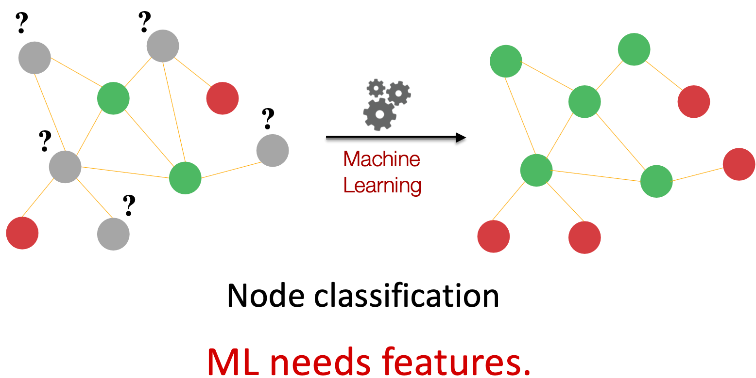
到目前为止定义的节点特征将允许区分上述示例中的节点。然而,到目前为止定义的特征还不能区分节点标签。
Link Prediction Task and Features
Task
任务是在现有链接的基础上预测新的链接。在测试时,对所有节点对(节点间无链接)进行排名,并预测 topK 节点对。关键是为一对节点设计特征。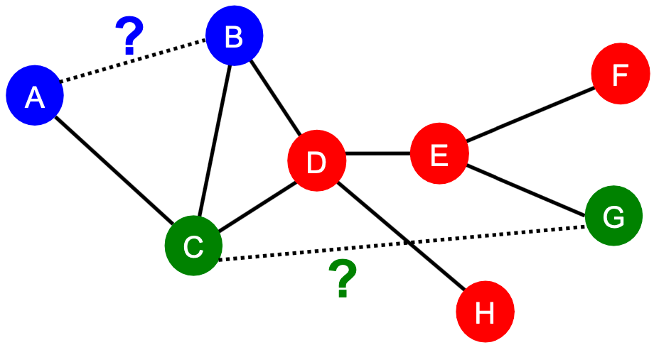
链接预测任务的两个公式:
- 随机缺失链接:
- 移除随机的一组链接,然后目标是预测它们;
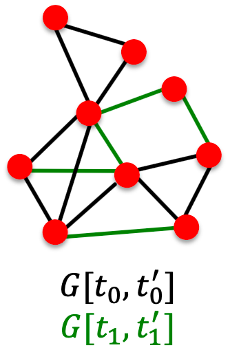
- 随时间推移的链接:
- 给定一个到时间
 的图
的图 ,输出预测会出现在
 中的链接的排名列表
 (不在
(不在 中);
中); - 评估:
 表示在测试
表示在测试 期间出现的新边数量,取
 的前
的前 个元素,计算正确的边数。
- 给定一个到时间
通过接近度(proximity)预测链路的方法论:
- 对于每对节点
 ,计算分数
,计算分数 ,如
,如 可为x与y的共同邻居的数量;
 - 通过对分数
 降序排序节点对
 ;
; - 预测top n对作为新的链接;
-
Features
Link-Level特征主要有以下三类:
distance-based 特征
- 局部邻域重叠
-
distance-based 特征
两个节点之间的最短路径距离:
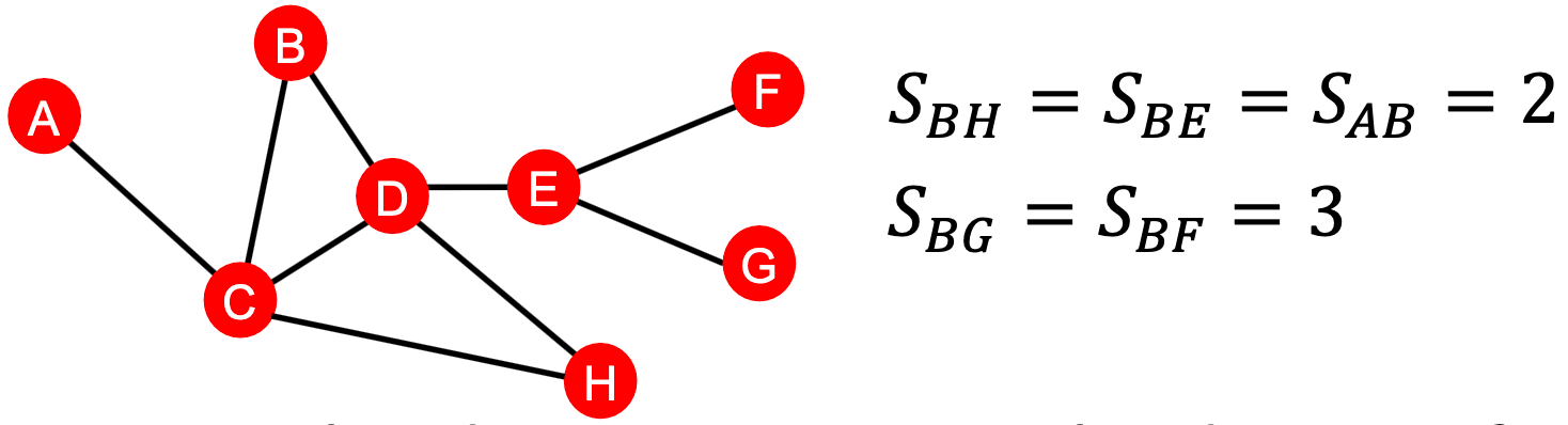
然而,这并没有反映出邻域重叠的程度,如节点对 共享2个邻居节点,而节点对
 和
和 仅共享1个邻居节点。
局部邻域重叠
捕获两个节点
 和
和 之间共享的邻居节点的数量:
 共同邻居:
 ,如
,如
- Jaccard’s 系数:
 ,如
,如
-
全局邻域重叠
局部邻域特征的局限性:如果两个节点没有任何共同的邻居,度量值总是0。然而,这两个节点在未来仍有可能被连接。
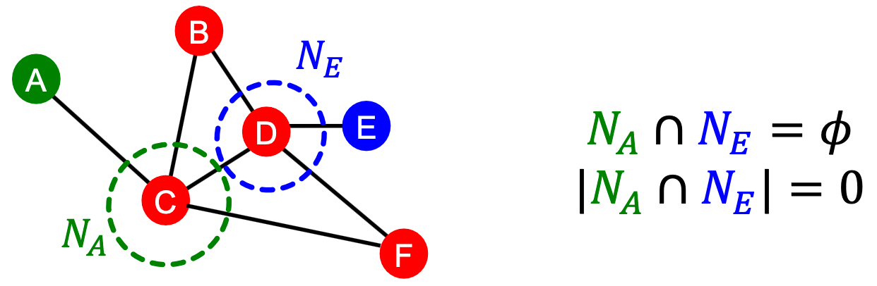
全局邻域重叠度量从全局图的角度解决了这一问题。
katz index:计算给定节点对之间所有长度的路径数。
Q:如何计算两节点之间的路径?使用图邻接矩阵的幂。
 表示节点
表示节点 与
与 之间长度为
之间长度为 的路径数
的路径数
下面证明
 表示节点
表示节点 与
与 之间长度为1的路径数(直接邻居)
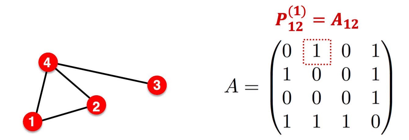
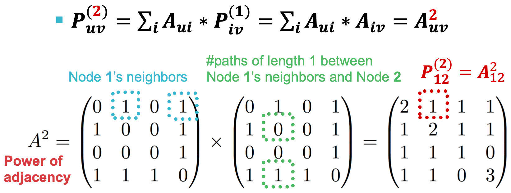
 表示节点
表示节点 与
与 之间长度为1的路径数(直接邻居)
 表示节点
表示节点 与
与 之间长度为2的路径数(邻居的邻居)
 表示节点
表示节点 与
与 之间长度为
之间长度为 的路径数
的路径数
 图中。
图中。
 ,如
,如
节点 与
与 之间的 Katz index 计算:所有路径长度的总和,
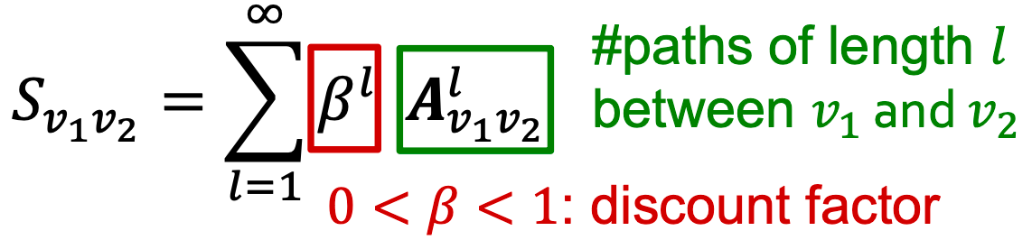
Katz index 矩阵以封闭形式计算: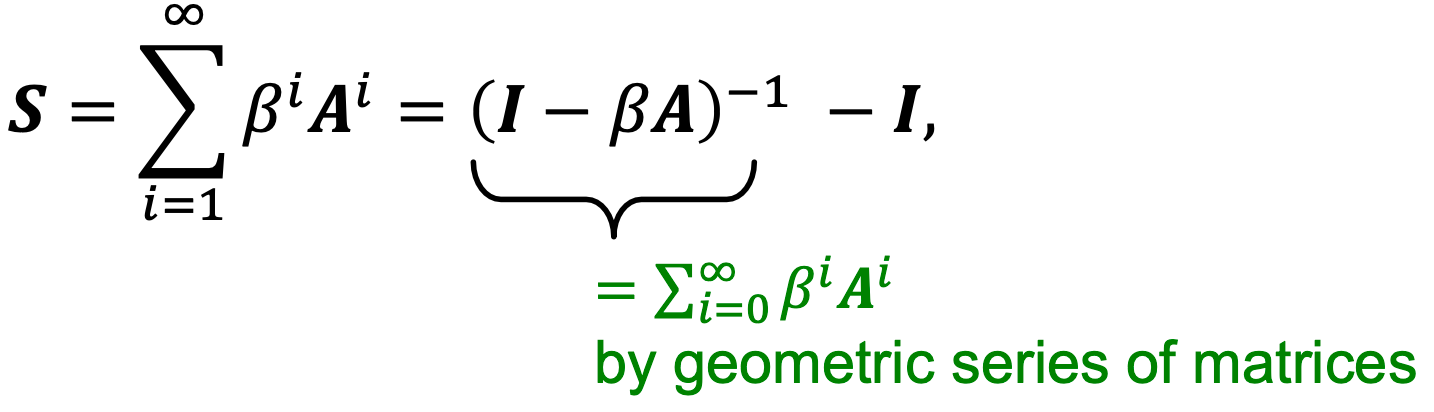
summary
- distance-based features:使用两个节点之间的最短路径长度,但捕捉不到邻域重叠结构;
- local neighborhood overlap:捕获两个节点共享的相邻节点的数量,当没有共享邻居节点时为零;
global neighborhood overlap:使用全局图结构给两个节点打分,Katz index 计数两个节点之间所有长度的路径数量。
Graph-Level Features and Graph Kernels
目标:我们想要能够描述整个图的结构的特征。
核方法在传统的ML中广泛用于图级预测,思想是设计核而不是特征向量。
核的介绍:核
 测量b/w数据的相似性
- 核矩阵
 必须是半正定的(如有正的特征值)
 - 存在特征表示
 ,使得
,使得
- 一旦定义了核,就可以使用现成的ML模型(如核SVM)进行预测
Graph kernels:测量两个图之间的相似性,如(1)Graphlet Kernel,(2)Weisfeiler-Lehman Kernel,(3)其他如Random-walk kernel,Shortest-path graph kernel等。
Graph kernels目标是设计图特征向量 ,主要思想是用Bag-of-Words (BoW)表示一个图。
BoW只是将单词计数作为文档的特性(没有考虑顺序),很自然扩展到一个图上,可将节点视为单词。因为两个图都有4个红节点,所以我们得到了两个不同图的相同特征向量。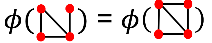
如果我们使用Bag的节点度,则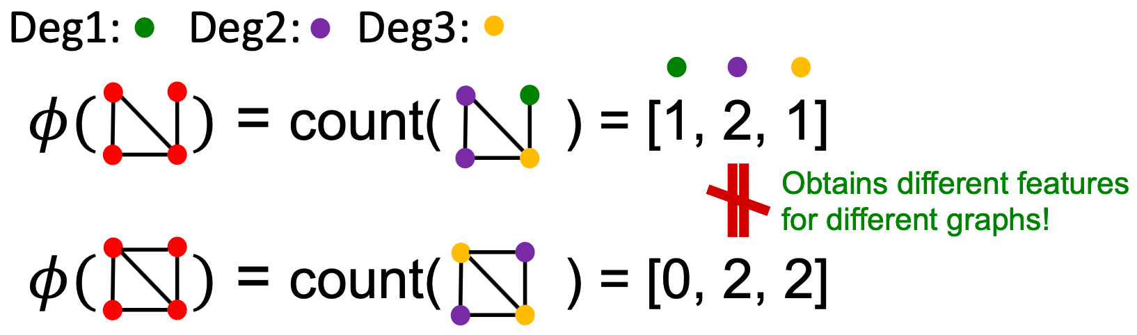
Graphlet核和Weisfeiler-Lehman (WL)核都使用Bag-of-表示图,其中比节点度更复杂!
Graphlet features
主要思想:计算图中不同graphlets的数量。
这里的graphlets定义与节点级特性略有不同:
- 这里的graphlets中的节点不需要连接(允许孤立节点);
- 这里的graphlets没有rooted。
设 是大小为
是大小为 的graphlets列表,
对于 ,有4个graphlets
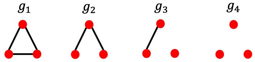
对于 ,有11个graphlets
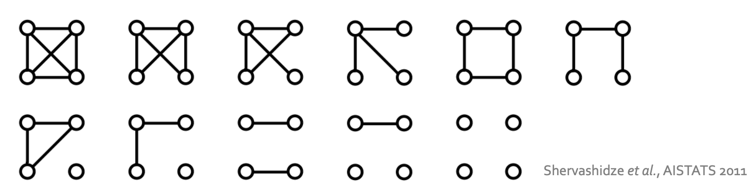
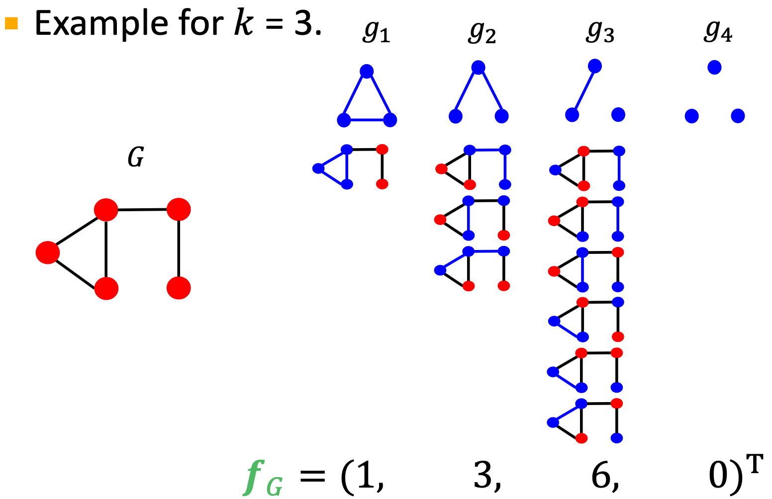
给定图 ,graphlet list
  ,定义graphlet 计数向量
 为
为
Graphlet Kernel
给定两个图 和
和 ,graphlet kernel计算为
 ,问题是
,问题是 和
和 的大小不同,这将极大地扭曲值。解决方法:标准化每个特征向量,即
 ,
, 。
。
Graph let kernel的局限性:计数graphlets代价高。
- 对大小为
 的图,通过枚举计数size-k graphlets需要
 ;
; - 这在最坏情况下是不可避免的,因为子图同构检验(判断一个图是否是另一个图的子图)是NP-hard;
如果图的节点度以
 为界,则存在
 算法来计数大小为
 的所有graphlets。
Weifeiler-Lehman Kernel
目标:设计一个有效的图特征描述
 .
.
想法:使用邻域结构迭代丰富节点词汇表。广义版的Bag of node degree,因为节点度是单跳(one-hop)的邻域信息。
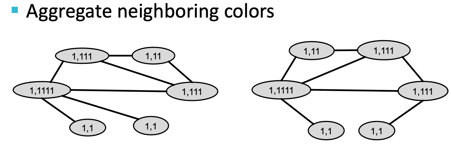
算法实现:Color refinement。Color refinement
给定包含一组节点
 的图
的图 ,给每个节点
 一初始颜色
一初始颜色 ,通过
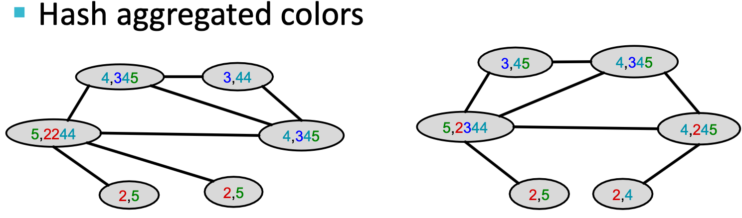
,通过 来迭代改进节点颜色,其中HASH映射不同输入到不同颜色,经过
 次迭代后,
次迭代后, 对𝐾-hop邻域结构进行了总结。
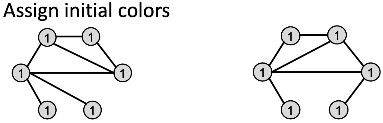
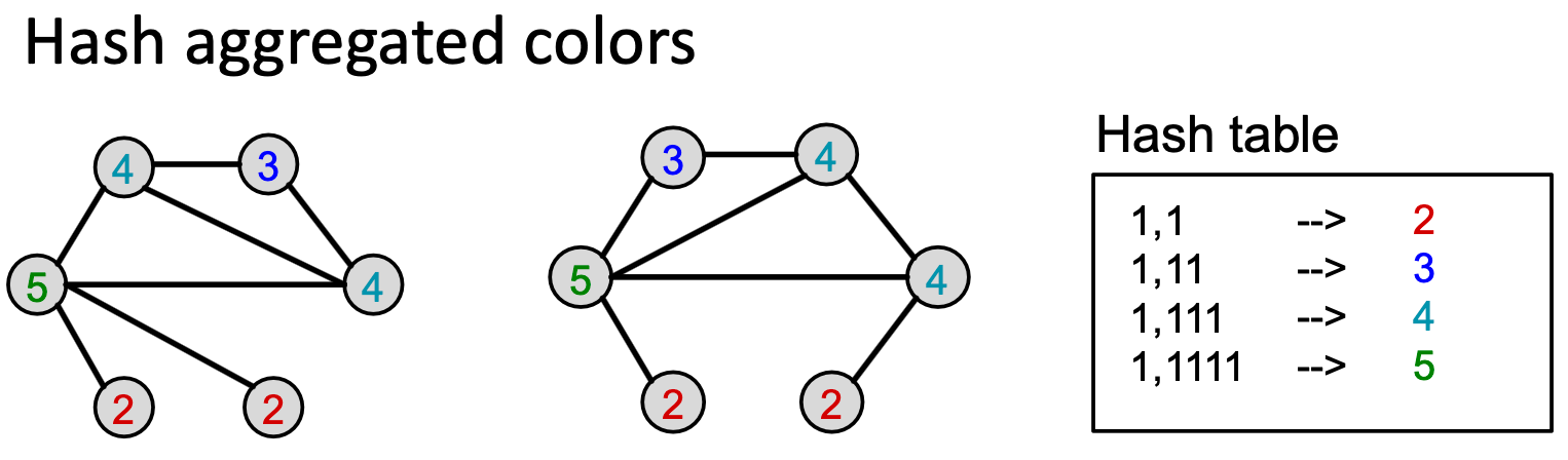
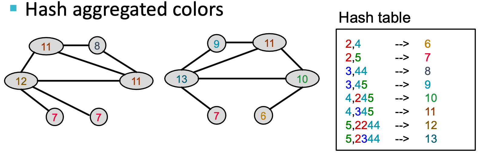
经过color refinement后,WL核对给定颜色的节点数量进行计数。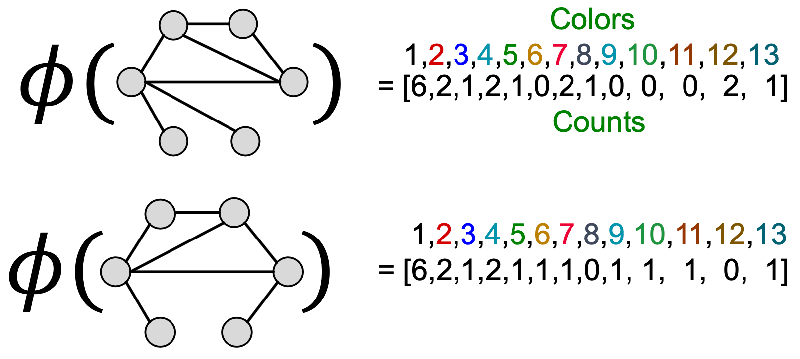
WL核值是通过颜色计数向量的内积来计算的: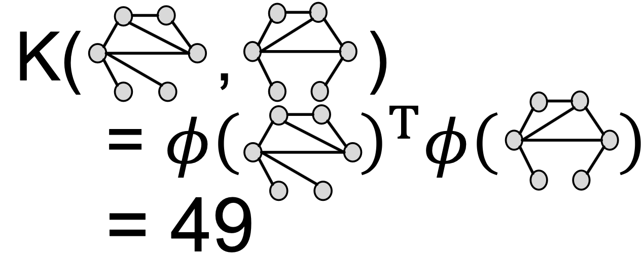
WL核具有较高的计算效率:color refinement每一步的时间复杂度在#(edges)中是线性的,因为它涉及到聚合邻近的颜色;
- 当计算一个核值时,只需要跟踪出现在两个图中的颜色。因此,#(colors)最多是节点的总数。
- 计算颜色需要线性时间w.r.t. #(节点)。「w.r.t. : with respect to 的缩写。是 关于;谈及,谈到的意思。」
-
Graph-level Features: Summary
Graphlet Kernel
- 图用Bag-of-graphlets表示;
- 计算复杂度高。
Weisfeiler-Lehman Kernel
手动设计特征 + ML model
图数据手动设计特征:
- Node-level:Node degree、centrality、clustering coefficient、graphlets
- Link-level:Distance-based feature、local/global neighborhood overlap
- Graph-level:Graphlet kernel、WL kernel

若有收获,就点个赞吧
0 人点赞
