- layout: post # 使用的布局(不需要改)title: 正确使用kmeans聚类的姿势 # 标题
subtitle: 正确使用kmeans聚类的姿势
date: 2019-09-06 # 时间
author: NSX # 作者
header-img: img/post-bg-2015.jpg #这篇文章标题背景图片
catalog: true # 是否归档
tags: #标签
- K-Means - 什么是聚类?
- K-means Clustering 如何在视觉上工作?
- K-Means伪代码
- 如何在 Python 中从头开始编写 K-means?
- 初始中心点怎么确定
- K值怎么确定
- 正确使用「K均值聚类」的Tips
- 小结
- 参考
layout: post # 使用的布局(不需要改)title: 正确使用kmeans聚类的姿势 # 标题
subtitle: 正确使用kmeans聚类的姿势
date: 2019-09-06 # 时间
author: NSX # 作者
header-img: img/post-bg-2015.jpg #这篇文章标题背景图片
catalog: true # 是否归档
tags: #标签
- K-Means
K-means 算法是一种基于相似属性将一组数据点划分为不同集群或组的方法。它是一种无监督学习算法,这意味着它不需要标记数据来查找数据集中的模式。
聚类的目标是将项目分成组,使得组中的对象比组外的对象更相似,我们可以在 k-means 中使用我们想要的任何相似度函数来比较两个点。
如何定义集群中的相似性?
比较两个数据点相似性的最常见和最直接的方法是使用距离。与使用勾股定理求对角线长度的方式相同,我们可以计算两个数据点之间的距离。
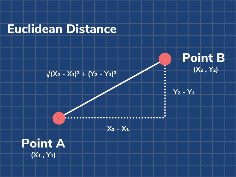
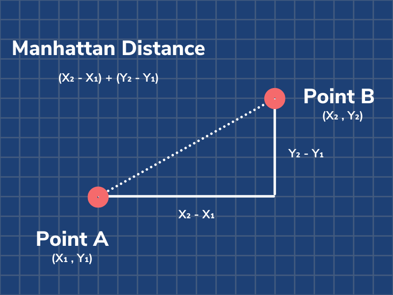
这种比较相似度的方法称为欧几里得距离。K-means 聚类中另一个常用的相似度函数称为曼哈顿距离。
这两个距离公式对用于聚类任务的各种数据集都很有效。然而,给定的相似度函数可能并非对数据点的每个分布都有效。这就提出了一个问题,“一个好的相似度函数的特性是什么?”。
良好相似函数的特征
可以使用三个基本属性来评估相似度函数是否良好。当然,还有更多的标准可以考虑,但这些是最重要的。在符号下方d(x,y)d ( x ,和) 读作“x 和 y 之间的距离”。
对称性: %20%3D%20d(y%2Cx)#card=math&code=d%28x%2Cy%29%20%3D%20d%28y%2Cx%29)
对称性很重要,否则我们可以说 A 看起来像 B,但 B 看起来一点也不像 A。
正可分离性:%20%3D%200%20%5Cquad%20if%20%5Cquad%20and%20%5Cquad%20only%20%5Cquad%20if%20%5Cquad%20x%3Dy#card=math&code=d%28x%2Cy%29%20%3D%200%20%5Cquad%20if%20%5Cquad%20and%20%5Cquad%20only%20%5Cquad%20if%20%5Cquad%20x%3Dy)
正可分性的属性很重要,因为否则可能会有两个不同的数据点 A 和 B,我们无法区分。
三角不等式:%20%5Cleq%20d(x%2Cz)%20%2B%20d(z%2Cy)#card=math&code=d%28x%2Cy%29%20%5Cleq%20d%28x%2Cz%29%20%2B%20d%28z%2Cy%29)
三角不等式很重要,否则我们可以说 A 看起来像 B,B 看起来像 C,但 A 看起来不像 C。
常用聚类方法概述
本文重点介绍 K 均值聚类,但这只是现有的众多聚类算法之一。
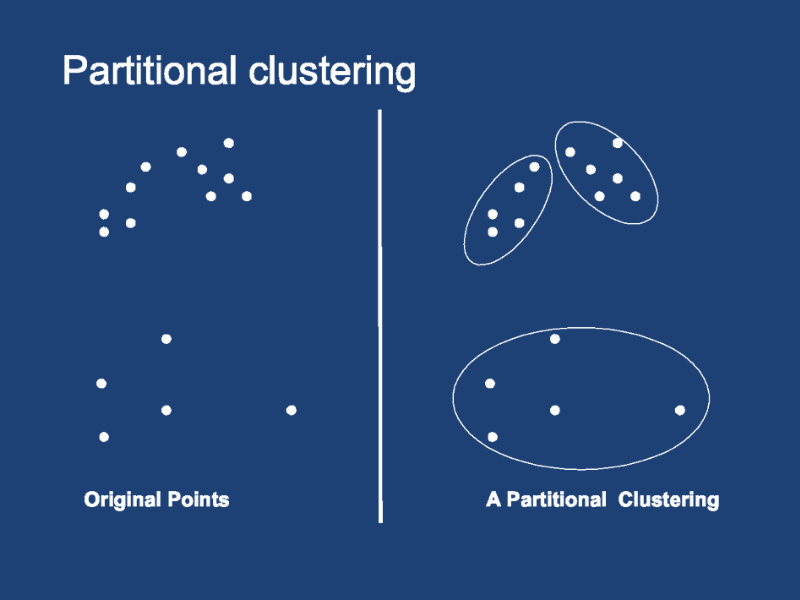
1.分区聚类
K-means 是分区聚类算法(也称为基于质心的聚类)的一个例子。这意味着它接受用户提供的集群数量k,并将数据划分为许多分区。在分区聚类中,每个数据点只能属于一个集群,任何集群都不能为空。
许多分区聚类算法是非确定性的。这意味着,即使您保持输入固定,每次运行算法时也可能最终得到不同的集群。
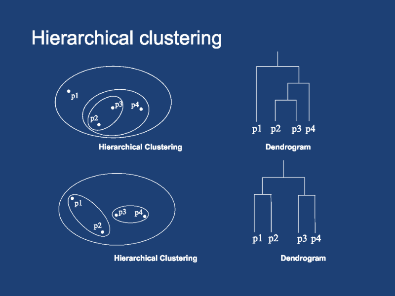
2.层次聚类
层次聚类下的算法通过自上而下或自下而上构建层次结构来将对象分配给集群。
自顶向下的方法称为分裂聚类。它的工作原理是从一个集群中的所有点开始,然后在每一步拆分最不相似的集群,直到每个数据点都在一个单独的集群中。
自底向上的方法称为凝聚聚类。这种方法迭代地合并集群中两个最相似的点,直到只有一个大集群。
与分区聚类方法不同,层次聚类是确定性的。这意味着集群分配在同一数据集上的运行之间不会有所不同。
自上而下和自下而上的方法都会产生一个基于树的点层次结构,称为 dendrogram。事实证明,此树状图可用于选择要使用的集群数量。您可以在任何深度切割树以生成不相交树的子集,每个树代表一个集群。
比较分区聚类和层次聚类
两种聚类方法各有优缺点。首先我们来看看使用K-means(partitional clustering)的优缺点。
| K-means 的优点 | K-means 的缺点 |
|---|---|
| 易于实施 | 难以预测聚类的数量(K-Value) |
| k-Means 可能比具有大量变量的层次聚类更快(如果 K 很小) | 初始种子对最终结果有很大影响 |
| k-Means 可能产生比层次聚类更紧密的聚类 | 数据的顺序对最终结果有影响 |
| 重新计算质心时,实例可以更改集群(移动到另一个集群) | 对缩放敏感:重新缩放数据集(标准化或标准化)将 完全改变结果。 |
现在,让我们来看看层次聚类的优点和缺点。
| 层次聚类的优点 | 层次聚类的缺点 |
|---|---|
| 输出比 k-means 返回的非结构化集群集信息更多的层次结构。 | 一旦一个点被分配给一个 集群,它就不能再四处移动了。 |
| 易于实施 | 时间复杂度:不适合大数据集 |
| 初始种子对最终结果有很大影响 | |
| 数据的顺序对最终结果有影响 |
我已经概述了两个聚类算法系列。还有其他类型的聚类算法我没有介绍,例如基于密度的聚类。有关聚类算法的更完整概述,请访问此资源。
K-means Clustering 如何在视觉上工作?
此可视化显示了使用 3 个集群运行的 k-means 算法。首先,初始化三个质心。这些是每个集群的初始中心,由蓝色、红色和绿色大点表示。
接下来,计算给定数据点与三个质心中的每一个之间的距离。这是针对所有数据点完成的。每个点都分配给它最接近的质心的集群。当我在可视化中单击重新分配点时会发生这种情况。
然后,通过对相应集群中每个数据点的坐标求平均值来重新计算质心。当我单击Update Centroids时会发生这种情况。
这个重新分配点和更新质心的过程一直持续到质心不再移动。
您可以使用此可视化自己直观地了解 k-means!在这里试试。
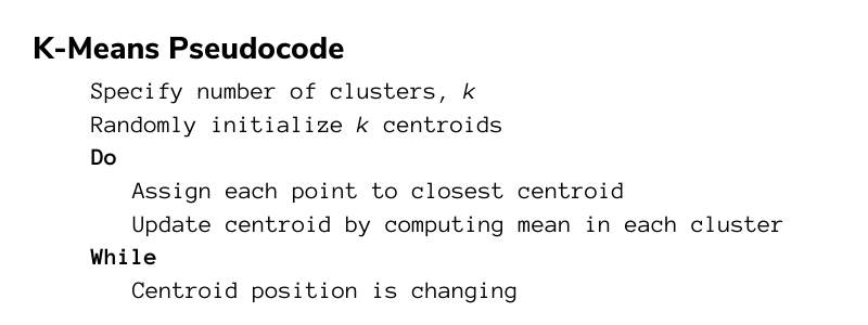
K-Means伪代码
K-Means聚类步骤是一个循环迭代的算法,非常简单易懂:
- 假定我们要对N个样本观测做聚类,要求聚为K类,首先选择K个点作为
初始中心点; - 接下来,按照
距离初始中心点最小的原则,把所有观测分到各中心点所在的类中; - 每类中有若干个观测,计算K个类中
所有样本点的均值,作为第二次迭代的K个中心点; - 然后根据这个中心重复第2、3步,直到
收敛(中心点不再改变或达到指定的迭代次数),聚类过程结束。
如何在 Python 中从头开始编写 K-means?
我们的 k-means 实现将分为五个辅助方法和一个运行算法的主循环。让我们一一介绍这些功能。
- 成对距离
- 初始化中心
- 更新分配
- 更新中心
- 计算损失
- 主循环
- 完整的实现
计算成对距离
def pairwise_dist(self, x, y):"""Args:x: N x D numpy arrayy: M x D numpy arrayReturn:dist: N x M array, where dist2[i, j] is the euclidean distance betweenx[i, :] and y[j, :]"""xSumSquare = np.sum(np.square(x),axis=1);ySumSquare = np.sum(np.square(y),axis=1);mul = np.dot(x, y.T);dists = np.sqrt(abs(xSumSquare[:, np.newaxis] + ySumSquare-2*mul))return dists
pairwise_dist 函数与前面描述的相似性函数等效。这是我们比较两点相似性的指标。在这里,我使用的是欧几里得距离。我使用的公式可能看起来与欧几里德距离函数的常规公式不同。这是因为我们正在执行矩阵操作,而不是使用两个单个向量。在这里深入阅读。
初始化中心
def _init_centers(self, points, K, **kwargs):"""Args:points: NxD numpy array, where N is # points and D is the dimensionalityK: number of clusterskwargs: any additional arguments you wantReturn:centers: K x D numpy array, the centers."""row, col = points.shaperetArr = np.empty([K, col])for number in range(K):randIndex = np.random.randint(row)retArr[number] = points[randIndex]return retArr
该函数接收点数组并随机选择其中的 K 个作为初始质心。该函数仅返回 K 个选定点。
更新分配
def _update_assignment(self, centers, points):"""Args:centers: KxD numpy array, where K is the number of clusters, and D is the dimensionpoints: NxD numpy array, the observationsReturn:cluster_idx: numpy array of length N, the cluster assignment for each pointHint: You could call pairwise_dist() function."""row, col = points.shapecluster_idx = np.empty([row])distances = self.pairwise_dist(points, centers)cluster_idx = np.argmin(distances, axis=1)return cluster_idx
更新分配函数负责选择每个点应该属于哪个集群。首先,我使用 pairwise_dist 函数计算每个点和每个质心之间的距离。然后,我得到每一行的最小距离的索引。最小距离的索引也是给定数据点的聚类分配索引,因为我们希望将每个点分配给最近的质心。
更新中心
def _update_centers(self, old_centers, cluster_idx, points):"""Args:old_centers: old centers KxD numpy array, where K is the number of clusters, and D is the dimensioncluster_idx: numpy array of length N, the cluster assignment for each pointpoints: NxD numpy array, the observationsReturn:centers: new centers, K x D numpy array, where K is the number of clusters, and D is the dimension."""K, D = old_centers.shapenew_centers = np.empty(old_centers.shape)for i in range(K):new_centers[i] = np.mean(points[cluster_idx == i], axis = 0)return new_centers
更新中心功能负责对属于给定集群的所有点进行平均。该平均值是相应聚类的新质心。该函数返回新中心的数组。
计算损失
def _get_loss(self, centers, cluster_idx, points):"""Args:centers: KxD numpy array, where K is the number of clusters, and D is the dimensioncluster_idx: numpy array of length N, the cluster assignment for each pointpoints: NxD numpy array, the observationsReturn:loss: a single float number, which is the objective function of KMeans."""dists = self.pairwise_dist(points, centers)loss = 0.0N, D = points.shapefor i in range(N):loss = loss + np.square(dists[i][cluster_idx[i]])return loss
损失函数是我们评估聚类算法性能的指标。我们的损失只是每个点与其聚类质心之间的平方距离之和。在我们的实现中,我们首先调用成对距离来获得每个点和每个中心之间的距离矩阵。我们使用 cluster_idx 为每个点选择与集群对应的适当距离2。
主循环
def __call__(self, points, K, max_iters=100, abs_tol=1e-16, rel_tol=1e-16, verbose=False, **kwargs):"""Args:points: NxD numpy array, where N is # points and D is the dimensionalityK: number of clustersmax_iters: maximum number of iterations (Hint: You could change it when debugging)abs_tol: convergence criteria w.r.t absolute change of lossrel_tol: convergence criteria w.r.t relative change of lossverbose: boolean to set whether method should print loss (Hint: helpful for debugging)kwargs: any additional arguments you wantReturn:cluster assignments: Nx1 int numpy arraycluster centers: K x D numpy array, the centersloss: final loss value of the objective function of KMeans"""centers = self._init_centers(points, K, **kwargs)for it in range(max_iters):cluster_idx = self._update_assignment(centers, points)centers = self._update_centers(centers, cluster_idx, points)loss = self._get_loss(centers, cluster_idx, points)K = centers.shape[0]if it:diff = np.abs(prev_loss - loss)if diff < abs_tol and diff / prev_loss < rel_tol:breakprev_loss = lossif verbose:print('iter %d, loss: %.4f' % (it, loss))return cluster_idx, centers, loss
现在,在主循环中,我们可以组合所有实用函数并实现伪代码。首先,中心用_init_centers随机初始化。然后,对于指定的迭代次数,我们重复update_assignment和update_centers步骤。每次迭代后,我们计算总损失并将其与之前的损失进行比较。如果差异小于我们的阈值,则算法执行完成。
完整的 K-Means 类实现
from __future__ import absolute_importfrom __future__ import print_functionfrom __future__ import divisionimport sysimport matplotlibimport numpy as npimport matplotlib.pyplot as pltfrom mpl_toolkits.mplot3d import axes3dfrom tqdm import tqdm# Load imageimport imageio# Set random seed so output is all samenp.random.seed(1)class KMeans(object):def __init__(self): # No need to implementpassdef pairwise_dist(self, x, y): # [5 pts]"""Args:x: N x D numpy arrayy: M x D numpy arrayReturn:dist: N x M array, where dist2[i, j] is the euclidean distance betweenx[i, :] and y[j, :]"""xSumSquare = np.sum(np.square(x),axis=1);ySumSquare = np.sum(np.square(y),axis=1);mul = np.dot(x, y.T);dists = np.sqrt(abs(xSumSquare[:, np.newaxis] + ySumSquare-2*mul))return distsdef _init_centers(self, points, K, **kwargs): # [5 pts]"""Args:points: NxD numpy array, where N is # points and D is the dimensionalityK: number of clusterskwargs: any additional arguments you wantReturn:centers: K x D numpy array, the centers."""row, col = points.shaperetArr = np.empty([K, col])for number in range(K):randIndex = np.random.randint(row)retArr[number] = points[randIndex]return retArrdef _update_assignment(self, centers, points): # [10 pts]"""Args:centers: KxD numpy array, where K is the number of clusters, and D is the dimensionpoints: NxD numpy array, the observationsReturn:cluster_idx: numpy array of length N, the cluster assignment for each pointHint: You could call pairwise_dist() function."""row, col = points.shapecluster_idx = np.empty([row])distances = self.pairwise_dist(points, centers)cluster_idx = np.argmin(distances, axis=1)return cluster_idxdef _update_centers(self, old_centers, cluster_idx, points): # [10 pts]"""Args:old_centers: old centers KxD numpy array, where K is the number of clusters, and D is the dimensioncluster_idx: numpy array of length N, the cluster assignment for each pointpoints: NxD numpy array, the observationsReturn:centers: new centers, K x D numpy array, where K is the number of clusters, and D is the dimension."""K, D = old_centers.shapenew_centers = np.empty(old_centers.shape)for i in range(K):new_centers[i] = np.mean(points[cluster_idx == i], axis = 0)return new_centersdef _get_loss(self, centers, cluster_idx, points): # [5 pts]"""Args:centers: KxD numpy array, where K is the number of clusters, and D is the dimensioncluster_idx: numpy array of length N, the cluster assignment for each pointpoints: NxD numpy array, the observationsReturn:loss: a single float number, which is the objective function of KMeans."""dists = self.pairwise_dist(points, centers)loss = 0.0N, D = points.shapefor i in range(N):loss = loss + np.square(dists[i][cluster_idx[i]])return lossdef __call__(self, points, K, max_iters=100, abs_tol=1e-16, rel_tol=1e-16, verbose=False, **kwargs):"""Args:points: NxD numpy array, where N is # points and D is the dimensionalityK: number of clustersmax_iters: maximum number of iterations (Hint: You could change it when debugging)abs_tol: convergence criteria w.r.t absolute change of lossrel_tol: convergence criteria w.r.t relative change of lossverbose: boolean to set whether method should print loss (Hint: helpful for debugging)kwargs: any additional arguments you wantReturn:cluster assignments: Nx1 int numpy arraycluster centers: K x D numpy array, the centersloss: final loss value of the objective function of KMeans"""centers = self._init_centers(points, K, **kwargs)for it in range(max_iters):cluster_idx = self._update_assignment(centers, points)centers = self._update_centers(centers, cluster_idx, points)loss = self._get_loss(centers, cluster_idx, points)K = centers.shape[0]if it:diff = np.abs(prev_loss - loss)if diff < abs_tol and diff / prev_loss < rel_tol:breakprev_loss = lossif verbose:print('iter %d, loss: %.4f' % (it, loss))return cluster_idx, centers, loss
这是我们在 Python 中完整的 K-means 类实现。我鼓励您复制此代码(或自己实现!)并在您自己的机器上运行它。这是巩固您对 K-means 算法理解的最佳方式。scikit-learn中的KMeans聚类实现
初始中心点怎么确定
在k-means算法步骤中,有两个地方降低了SSE:
- 把样本点分到最近邻的簇中,这样会降低SSE的值;
- 重新优化聚类中心点,进一步的减小了SSE。
这样的重复迭代、不断优化,会找到局部最优解(局部最小的SSE),如果想要找到全局最优解需要找到合理的初始聚类中心。
那合理的初始中心怎么选?
方法有很多,譬如先随便选个点作为第1个初始中心C1,接下来计算所有样本点与C1的距离,距离最大的被选为下一个中心C2,直到选完K个中心。这个算法叫做K-Means++,可以理解为 K-Means的改进版,它可以能有效地解决初始中心的选取问题,但无法解决离群点问题。
K值怎么确定
使用 K 均值算法,性能可能会因您使用的集群数量而有很大差异。要知道,K设置得越大,样本划分得就越细,每个簇的聚合程度就越高,误差平方和SSE自然就越小。所以不能单纯像选择初始点那样,用不同的K来做尝试,选择SSE最小的聚类结果对应的K值,因为这样选出来的肯定是你尝试的那些K值中最大的那个。
“手肘法”(Elbow Method)
为了使用肘部方法,您只需多次运行 K-means 算法,每次迭代将聚类数增加一个。记录每次迭代的损失,然后制作 num cluster vs loss 的折线图。
下面是肘部方法的简单实现:
def find_optimal_num_clusters(self, data, max_K=15):"""Plots loss values for different number of clusters in K-MeansArgs:image: input image of shape(H, W, 3)max_K: number of clustersReturn:None (plot loss values against number of clusters)"""y_val = np.empty(max_K)for i in range(max_K):cluster_idx, centers, y_val[i] = KMeans()(data, i + 1)plt.plot(np.arange(max_K) + 1, y_val)plt.show()return y_val
from sklearn.cluster import KMeansloss = []for i in range(1, 10):kmeans = KMeans(n_clusters=i, max_iter=100).fit(p_list)loss.append(kmeans.inertia_ / point_number / K)plt.plot(range(1, 10), loss)plt.show()
运行此方法将输出一个类似于您在下面看到的图:
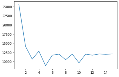
现在,为了选择正确数量的簇,我们进行目视检查。损耗曲线开始弯曲的点称为 肘点。肘点代表误差和聚类数量之间的合理权衡。在此示例中,肘点位于x = 3 处。这意味着最佳聚类数为 3。
轮廓系数
数据的平均轮廓是评估集群自然数的另一个有用标准。数据实例的轮廓是衡量它与集群内数据匹配程度以及与相邻集群数据匹配程度的度量。
轮廓值是衡量一个对象与其自己的集群(内聚)相比其他集群(分离)的相似程度。轮廓范围从 -1 到 +1,其中高值表示对象与其自己的集群匹配良好,而与相邻集群匹配不佳。如果大多数对象具有较高的值,则集群配置是合适的。如果许多点具有低值或负值,则聚类配置可能具有过多或过少的聚类。
如果您想实现用于聚类分析的轮廓系数,我建议使用 scikit-learn。访问此资源以获取有关实施的完整指南。
正确使用「K均值聚类」的Tips
- 输入数据一般需要做缩放,如标准化。原因很简单,K均值是建立在距离度量上的,因此不同变量间如果维度差别过大,可能会造成少数变量“施加了过高的影响而造成垄断”。
- 输出结果非固定,多次运行结果可能不同。首先要意识到K-means中是有随机性的,从初始化到收敛结果往往不同。一种看法是强行固定随机性,比如设定sklearn中的random state为固定值。另一种看法是,如果你的K均值结果总在大幅度变化,比如不同簇中的数据量在多次运行中变化很大,那么K均值不适合你的数据,不要试图稳定结果 [2]。
- 运行时间往往可以得到优化,选择最优的工具库。基本上现在的K均值实现都是K-means++,速度都不错。但当数据量过大时,依然可以使用其他方法,如MiniBatchKMeans [3]。上百万个数据点往往可以在数秒钟内完成聚类,推荐Sklearn的实现。
- 高维数据上的有效性有限。建立在距离度量上的算法一般都有类似的问题,那就是在高维空间中距离的意义有了变化,且并非所有维度都有意义。这种情况下,K均值的结果往往不好,而通过划分子空间的算法(sub-spacing method)效果可能更好。
- 运行效率与性能之间的取舍。
小结
因此不难看出,K-Means优点在于原理简单,运行速度快且容易实现,能够处理的数据量大。
当然,也有一些缺点:
- 在高维上可能不是最佳选项
- K值、初始点的选取不好确定;
- 得到的结果只是局部最优;
- 受离群值影响大。
一个比较粗浅的结论是,在数据量不大时,可以优先尝试其他算法。当数据量过大时,可以试试HDBSCAN。仅当数据量巨大,且无法降维或者降低数量时,再尝试使用K均值。
参考

若有收获,就点个赞吧
0 人点赞
