数据可视化
介绍一种”凹凸图(bump charts)“的绘制方法,其绘图函数主要来自R包-ggbump,主要内容如下:
- R-ggbump包基本绘图简介
- R-ggbump包实例演示
R-ggbump包基本绘图函数简介
R-ggbump包主要包含:geom_bump()和geom_sigmoid(),两个函数主要绘制随时间变化的平滑曲线排名图,内置参数也几乎相同,如下:
其官网(https://github.com/davidsjoberg/ggbump)提供的例子如下(部分):( mapping = NULL,data = NULL,geom = "line",position = "identity",na.rm = FALSE,show.legend = NA,smooth = 8,direction = "x",inherit.aes = TRUE,...)
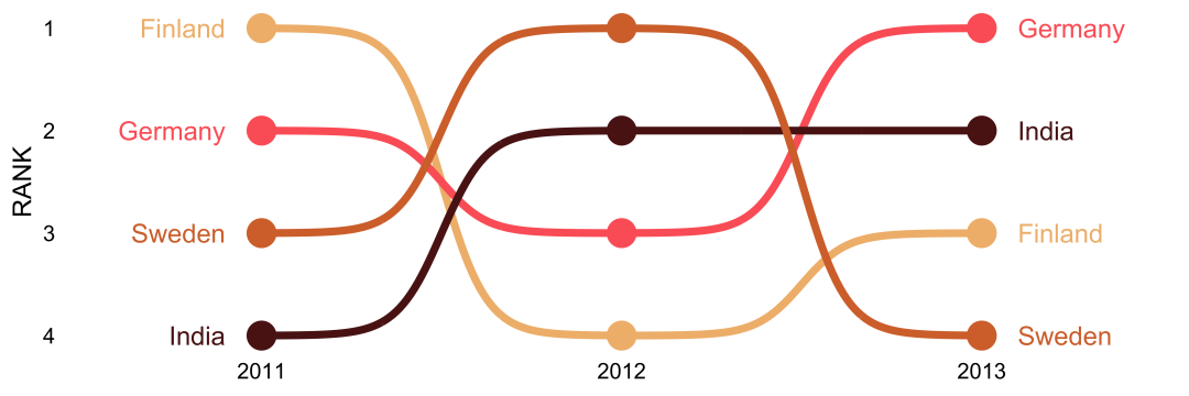
Example Of geom_bump()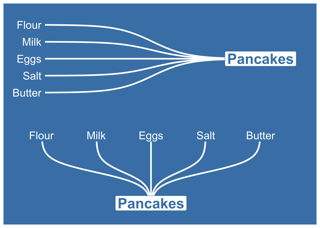
Example Of geom_sigmoid()
从以上也可以看出两个绘图函数所绘制的图形属于同一类别,下面通过实例数据进行两个绘图函数的理解。R-ggbump包实例演示
geom_bump()绘图函数「样例一:」
直接构造数据并对结果继续美化操作,代码如下:
可以看到仅使用library(tidyverse)library(ggtext)library(hrbrthemes)library(wesanderson)library(LaCroixColoR)library(RColorBrewer)library(ggbump)#数据构建和处理test_01 <- tibble(country = c("India", "India", "India", "Sweden", "Sweden", "Sweden", "Germany", "Germany", "Germany", "Finland", "Finland", "Finland"),year = c(2011, 2012, 2013, 2011, 2012, 2013, 2011, 2012, 2013, 2011, 2012, 2013),value = c(492, 246, 246, 369, 123, 492, 246, 369, 123, 123, 492, 369))test_01_plot <- test_01 %>% group_by(year) %>% mutate(rank=rank(value, ties.method = "random")) %>% ungroup#可视化绘制charts01_cus <- ggplot(data = test_01_plot,aes(x = year,y = rank,color=country))+ggbump::geom_bump(size=2,smooth = 8) +#添加圆点geom_point(size=8)+# 添加文本信息geom_text(data = test_01_plot %>% filter(year==min(year)),aes(x=year-.1,label=country),size=6,fontface="bold",hjust = 1) +geom_text(data = test_01_plot %>% filter(year == max(year)),aes(x = year + .1, label = country), size = 6,fontface="bold",hjust = 0) +#修改刻度scale_x_continuous(limits = c(2010.6, 2013.4),breaks = seq(2011, 2013, 1)) +scale_color_manual(values = lacroix_palette("Pamplemousse", type = "discrete"))+labs(title = "Example of <span style='color:#D20F26'>ggbump::geom_bump function</span>",subtitle = "processed charts with <span style='color:#1A73E8'>geom_bump()</span>",caption = "Visualization by <span style='color:#DD6449'>DataCharm</span>")+hrbrthemes::theme_ft_rc(base_family = "Roboto Condensed") +theme(plot.title = element_markdown(hjust = 0.5,vjust = .5,color = "black",size = 20, margin = margin(t = 1, b = 12)),plot.subtitle = element_markdown(hjust = 0,vjust = .5,size=12),plot.caption = element_markdown(face = 'bold',size = 10),legend.position = "none",panel.grid.major = element_blank(),panel.grid.minor = element_blank())+scale_y_reverse()
geom_bump()即可绘制,到这里使用了更多的绘图函数和主题、样式等设置语句对其进行美化操作,可视化结果如下: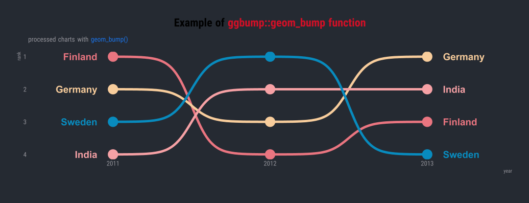
Exercise Of geom_bump()「样例二:」
第二个小例子,通过构建虚拟数据进行可视化结果绘制,如下: ```r读入数据
library(readxl)
df<-read_excel(“rank_data.xlsx”)
定义颜色
cols <- c( “#882B1A”, “#676564”, “#E8751A”, “#779AC4”, “#646E3F”, “#9D49B9”, “#C09F2F”, “#65955B”, “#284D95”,”#B34525”)
可视化绘制
charts02_cus <- ggplot(data = df,aes(x = race_num,y = rank,color=team_name,group=team_name)) + geom_bump(smooth = 7, size = 2.5) + geom_point(data = df %>% filter(race_num == 1),size = 5) + geom_point(data = df %>% filter(race_num == 7),size = 5, shape = 21, fill = “black”, stroke = 2) + geom_text(data = df %>% filter(race_num == 7),aes(x = 7.12,label = team_name), family = “Cinzel”,fontface = ‘bold’,size = 4, hjust = 0) +
添加序号
geom_point(data = tibble(x = .8, y = 1:10), aes(x = x, y = y), inherit.aes = F,shape=21,color = “grey95”,size = 5,stroke = 1.) + geom_text(data = tibble(x = .8, y = 1:10), aes(x = x, y = y, label = y), inherit.aes = F,size=2.5,fontface = ‘bold’, color = “grey95”)+ coord_cartesian(clip = “off”) + scale_x_continuous( expand = c(.01, .01), limits = c(.8, 8.1), breaks = 1:7, labels = c(“Begain”,glue::glue(“Race {1:5}”), “Finish”), sec.axis = dup_axis() ) + scale_y_reverse( expand = c(.05, .05), breaks = 1:16 ) + scale_color_manual( values = cols, guide = F ) + labs(x=””,y=””, title = “Example of ggbump::geom_bump() function“, subtitle = “processed charts with geom_bump()“, caption = “Visualization by DataCharm“)+ theme( plot.title = element_markdown(hjust = 0.5,vjust = .5,color = “gray50”,face = ‘bold’, size = 20, margin = margin(t = 1, b = 12)), plot.subtitle = element_markdown(hjust = 0,vjust = .5,size=12,color = “gray50”), plot.caption = element_markdown(face = ‘bold’,size = 10), plot.background = element_rect(fill = “black”, color = “black”), panel.background = element_rect(fill = “black”, color = “black”), panel.grid.major = element_blank(), panel.grid.minor = element_blank(), axis.text.x.top = element_text(size = 9,color = “grey95”,family = “Cinzel”,face = ‘bold’), axis.text.y.left = element_blank(), axis.ticks = element_blank() )
(这里涉及到很多关于主题设置的语句)<br />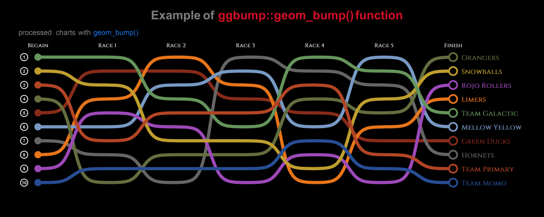<br />Exercise2 Of geom_bump<a name="zvf7Z"></a>### `geom_sigmoid()`绘图函数对于该函数,还是通过构建数据进行绘制:```rdata_test <- tibble(x = c(0.5,0.5,1,1,1,1,1,1),xend = c(1, 1, 3, 3, 3 ,3, 3, 3),y = c(4, 4, 6, 6, 6, 2, 2, 2),yend = c(6,2,7,6,5,3,2,1),group = c("Python","R","Numpy","Pandas","Matplolib","Dplyr","Data.table","Ggplot2"))#可视化绘制charts04_cus <- ggplot(data_test) +geom_sigmoid(data = data_test %>% filter(xend < 3),aes(x = x, y = y, xend = xend, yend = yend, group = factor(group)),direction = "x", color = "#cb7575", size = 2, smooth = 6) +geom_sigmoid(data = data_test %>% filter(group %in% c("Numpy","Pandas","Matplolib")),aes(x = x, xend = xend, y = y, yend = yend, group=group),direction = "x",color = "#cb7575", size = 2, smooth = 12) +geom_sigmoid(data = data_test %>% filter(y==2),aes(x = x, xend = xend, y = y, yend = yend, group=group),direction = "x",color = "#cb7575", size = 2, smooth = 11) +geom_label(data = tibble(x = 0.1, y = 4, label = "DataScience"),aes(x, y, label = label), inherit.aes = F, size = 10, color = "white",fill = "#004E66",family = "Cinzel",nudge_x = -.15) +geom_label(data = data_test %>% filter(xend < 3),aes(x = xend, y = yend, label = group),inherit.aes = F, size = 8,color = "white", fill = "#004E66", family = "Cinzel",hjust=0.5,nudge_y = .45,nudge_x = .3)+geom_label(data = data_test %>% filter(xend == 3),aes(x = xend, y = yend, label = group),inherit.aes = F, size = 7,color = "white", fill = "#004E66", family = "Cinzel",hjust=0) +labs(x="",y="",title = "Example of <span style='color:#D20F26'>ggbump::geom_sigmoid() function</span>",subtitle = "processed charts with <span style='color:#1A73E8'>geom_sigmoid()</span>",caption = "Visualization by <span style='color:#DD6449'>DataCharm</span>")+scale_x_continuous(limits = c(-.5,4)) +theme(plot.title = element_markdown(hjust = 0.5,vjust = .5,color = "gray50",face = 'bold',size = 20, margin = margin(t = 1, b = 12)),plot.subtitle = element_markdown(hjust = 0,vjust = .5,size=12,color = "gray50"),plot.caption = element_markdown(face = 'bold',size = 10),panel.grid = element_blank(),axis.line = element_blank(),axis.ticks = element_blank(),axis.text.y = element_blank(),axis.title.y = element_blank(),axis.text.x = element_blank(),panel.background = element_rect(fill = "#353848"),plot.background = element_rect(fill = "#353848",colour = "#353848"))
(使用了很多常用的主题设置语句)
Exercise Of geom_sigmoid

若有收获,就点个赞吧
0 人点赞
