绘图技巧 - 绘图技巧 | 快速绘制矩阵可视化统计图表技巧 - 《AI》

R-GGally包简介
- 官网
- 主要绘图函数简介
R-GGally包主要函数示例

数据科学
用可视化方式展现变量之间的关系。R-GGally包就可以轻松绘制配对图矩阵、散点图矩阵、平行坐标图和生存图等。主要内容如下：

R-GGally包简介
R-GGally包主要函数示例

R-GGally包简介
作为R-ggplot2的拓展包，其可以通过添加定义好的绘图函数绘制例如散点图矩阵、平行坐标图等统计图表。

官网
https://ggobi.github.io/ggally/index.html

主要绘图函数简介
ggmatrix()：用于管理矩阵状布局中的多图的绘图函数，其可适应任何数量的行和列。
ggpairs()：作为ggmatrix()的一种特殊形式，可实现对多元数据进行成对比较。默认情况下，ggpairs(): 提供每对列的两次不同比较，并沿对角线显示相应变量的密度或计数。通过不同的参数设置，可将对角线替换为轴值或者变量标签。
ggduo()：在绘图矩阵中用于显示两个分组数据，比较适用于多时间序列分析和回归分析。
ggally_*()：用于绘制多种高级图表。
ggbivariate()：用于地绘制一个结果和几个解释变量之间的双变量关系的可视化图。
ggnostic()：用于显示每个给定解释变量的完整模型诊断。
ggscatmat()：用于数字矩阵图绘制。
ggtable()：用于绘制绘制离散变量的交叉表。
ggcoef_model()：用于绘制模型的系数。
ggnetworkmap()：用于绘制各种精美的地图。

以上就是R-GGally包较为常用的绘图包。

R-GGally包主要函数示例

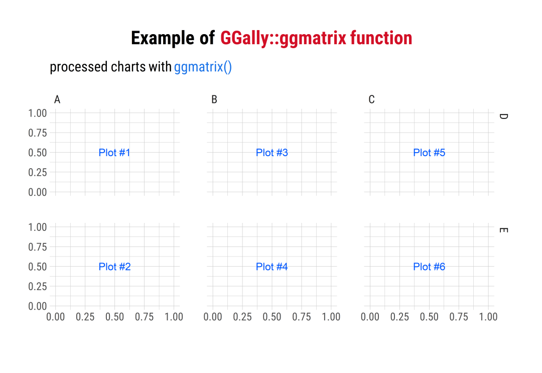
`ggmatrix()`绘图函数

plotList <- list()
for (i in 1:6) {
  plotList[[i]] <- ggally_text(paste("Plot #", i, sep = ""),color = I("#0057FF"))
}
#可视化绘制
ggmatrix <- GGally::ggmatrix(
      plotList,
      nrow = 2, ncol = 3,
      xAxisLabels = c("A", "B", "C"),
      yAxisLabels = c("D", "E"),
      title = "Matrix Title",
      byrow = FALSE) +
    labs(
        title = "Example of <span style='color:#D20F26'>GGally::ggmatrix function</span>",
        subtitle = "processed charts with <span style='color:#1A73E8'>ggmatrix()</span>",
        caption = "Visualization by <span style='color:#DD6449'>DataCharm</span>") +
    hrbrthemes::theme_ipsum(base_family = "Roboto Condensed") +
    theme(
    plot.title = element_markdown(hjust = 0.5,vjust = .5,color = "black",face = 'bold',
                                  size = 20, margin = margin(t = 1, b = 12)),
    plot.subtitle = element_markdown(hjust = 0,vjust = .5,size=15),
    plot.caption = element_markdown(face = 'bold',size = 12))

Example of ggmatrix

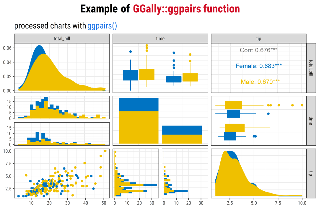
`ggpairs()`绘图函数

data(tips, package = "reshape")
ggpairs <- GGally::ggpairs(tips, mapping = aes(fill = sex,color=sex), 
                   columns = c("total_bill", "time", "tip")) +
  ggsci::scale_fill_jco() +
  ggsci::scale_color_jco() +
  labs(
        title = "Example of <span style='color:#D20F26'>GGally::ggpairs function</span>",
        subtitle = "processed charts with <span style='color:#1A73E8'>ggpairs()</span>",
        caption = "Visualization by <span style='color:#DD6449'>DataCharm</span>") +
    #hrbrthemes::theme_ipsum(base_family = "Roboto Condensed") +
    theme_bw(base_family = "Roboto Condensed")+
    theme(
    plot.title = element_markdown(hjust = 0.5,vjust = .5,color = "black",face = 'bold',
                                  size = 20, margin = margin(t = 1, b = 12)),
    plot.subtitle = element_markdown(hjust = 0,vjust = .5,size=15),
    plot.caption = element_markdown(face = 'bold',size = 12))

Example of ggpairs

ggally_*系列

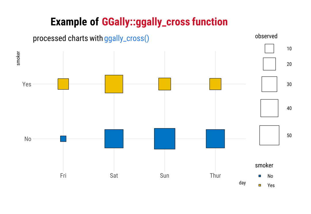
`ggally_cross()`

plot01 <- ggally_cross(tips, aes(x = day, y = smoker, fill = smoker)) +
   ggsci::scale_fill_jco() +
  labs(
        title = "Example of <span style='color:#D20F26'>GGally::ggally_cross function</span>",
        subtitle = "processed charts with <span style='color:#1A73E8'>ggally_cross()</span>",
        caption = "Visualization by <span style='color:#DD6449'>DataCharm</span>") +
    hrbrthemes::theme_ipsum(base_family = "Roboto Condensed") +
    theme(
    plot.title = element_markdown(hjust = 0.5,vjust = .5,color = "black",face = 'bold',
                                  size = 20, margin = margin(t = 1, b = 12)),
    plot.subtitle = element_markdown(hjust = 0,vjust = .5,size=15),
    plot.caption = element_markdown(face = 'bold',size = 12))

Example of ggally_cross

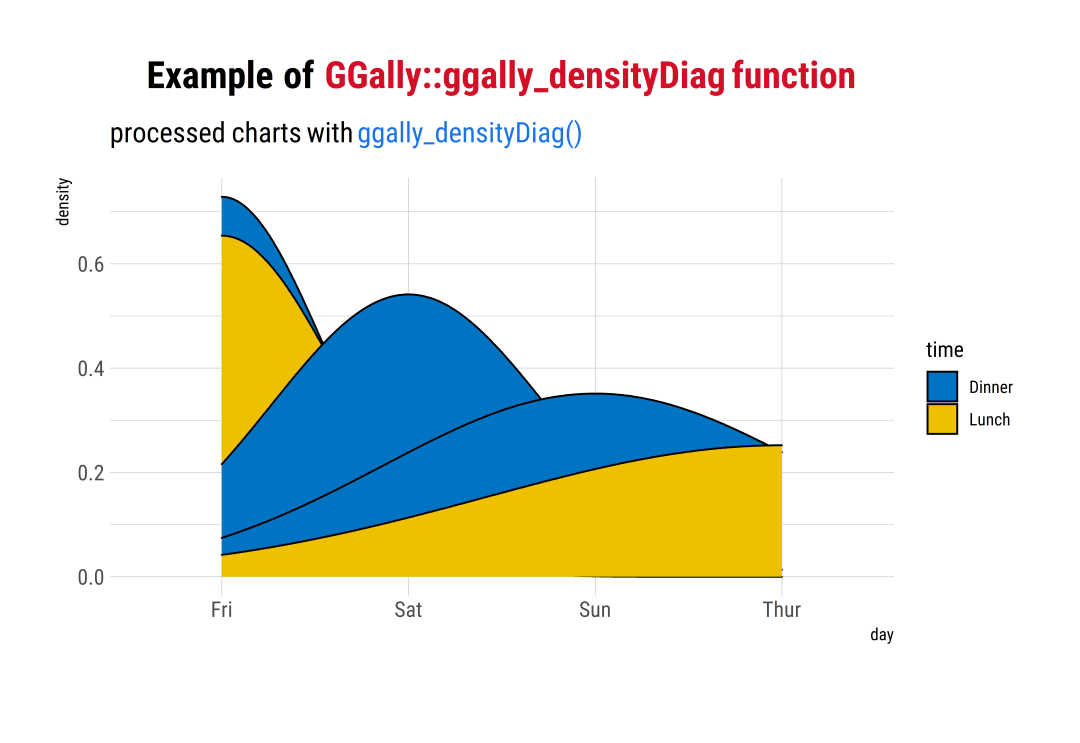
`ggally_densityDiag()`

plot02 <- ggally_densityDiag(tips, aes(x = day, fill = time)) +
  ggsci::scale_fill_jco() +
  labs(
        title = "Example of <span style='color:#D20F26'>GGally::ggally_densityDiag function</span>",
        subtitle = "processed charts with <span style='color:#1A73E8'>ggally_densityDiag()</span>",
        caption = "Visualization by <span style='color:#DD6449'>DataCharm</span>") +
    hrbrthemes::theme_ipsum(base_family = "Roboto Condensed") +
    theme(
    plot.title = element_markdown(hjust = 0.5,vjust = .5,color = "black",face = 'bold',
                                  size = 20, margin = margin(t = 1, b = 12)),
    plot.subtitle = element_markdown(hjust = 0,vjust = .5,size=15),
    plot.caption = element_markdown(face = 'bold',size = 12))

Example of ggally_densityDiag

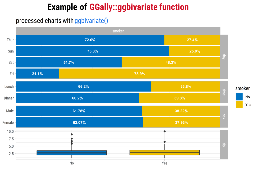
`ggbivariate()`绘图函数

ggbivariate <- ggbivariate(tips, outcome = "smoker", 
                           explanatory = c("day", "time", "sex", "tip"),
                           rowbar_args = list(
                                            colour = "white",
                                            size = 3,
                                            fontface = "bold",
                                            label_format = scales::label_percent(accurary = 1)
                                          )) +
  ggsci::scale_fill_jco() +
  labs(
        title = "Example of <span style='color:#D20F26'>GGally::ggbivariate function</span>",
        subtitle = "processed charts with <span style='color:#1A73E8'>ggbivariate()</span>",
        caption = "Visualization by <span style='color:#DD6449'>DataCharm</span>") +
    #hrbrthemes::theme_ipsum(base_family = "Roboto Condensed") +
    theme_light(base_family = "Roboto Condensed") +
    theme(
    plot.title = element_markdown(hjust = 0.5,vjust = .5,color = "black",face = 'bold',
                                  size = 20, margin = margin(t = 1, b = 12)),
    plot.subtitle = element_markdown(hjust = 0,vjust = .5,size=15),
    plot.caption = element_markdown(face = 'bold',size = 12))

Example of ggbivariate

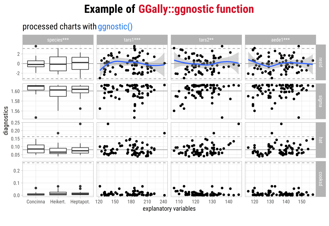
`ggnostic()`绘图函数

# 构建模型
flea_model <- step(lm(head ~ ., data = flea), trace = FALSE)
ggnostic <- ggnostic(flea_model) +
  labs(
        title = "Example of <span style='color:#D20F26'>GGally::ggnostic function</span>",
        subtitle = "processed charts with <span style='color:#1A73E8'>ggnostic()</span>",
        caption = "Visualization by <span style='color:#DD6449'>DataCharm</span>") +
    #hrbrthemes::theme_ipsum(base_family = "Roboto Condensed") +
    theme_light(base_family = "Roboto Condensed") +
    theme(
    plot.title = element_markdown(hjust = 0.5,vjust = .5,color = "black",face = 'bold',
                                  size = 20, margin = margin(t = 1, b = 12)),
    plot.subtitle = element_markdown(hjust = 0,vjust = .5,size=15),
    plot.caption = element_markdown(face = 'bold',size = 12))

Example of ggnostic

`ggcoef_model()`绘图函数

library(labelled)
# 数据处理
tips_labelled <- tips %>%
  labelled::set_variable_labels(
    day = "Day of the week",
    time = "Lunch or Dinner",
    total_bill = "Bill's total"
  )
mod_labelled <- lm(tip ~ day + time + total_bill, data = tips_labelled)
ggcoef_model <- ggcoef_model(mod_labelled,colour_guide = TRUE) +
ggsci::scale_color_aaas() +
   labs(
        title = "Example of <span style='color:#D20F26'>GGally::ggcoef_model function</span>",
        subtitle = "processed charts with <span style='color:#1A73E8'>ggcoef_model()</span>",
        caption = "Visualization by <span style='color:#DD6449'>DataCharm</span>") +
    #hrbrthemes::theme_ipsum(base_family = "Roboto Condensed") +
    theme_light(base_family = "Roboto Condensed") +
    theme(
    plot.title = element_markdown(hjust = 0.5,vjust = .5,color = "black",face = 'bold',
                                  size = 20, margin = margin(t = 1, b = 12)),
    plot.subtitle = element_markdown(hjust = 0,vjust = .5,size=15),
    plot.caption = element_markdown(face = 'bold',size = 12))

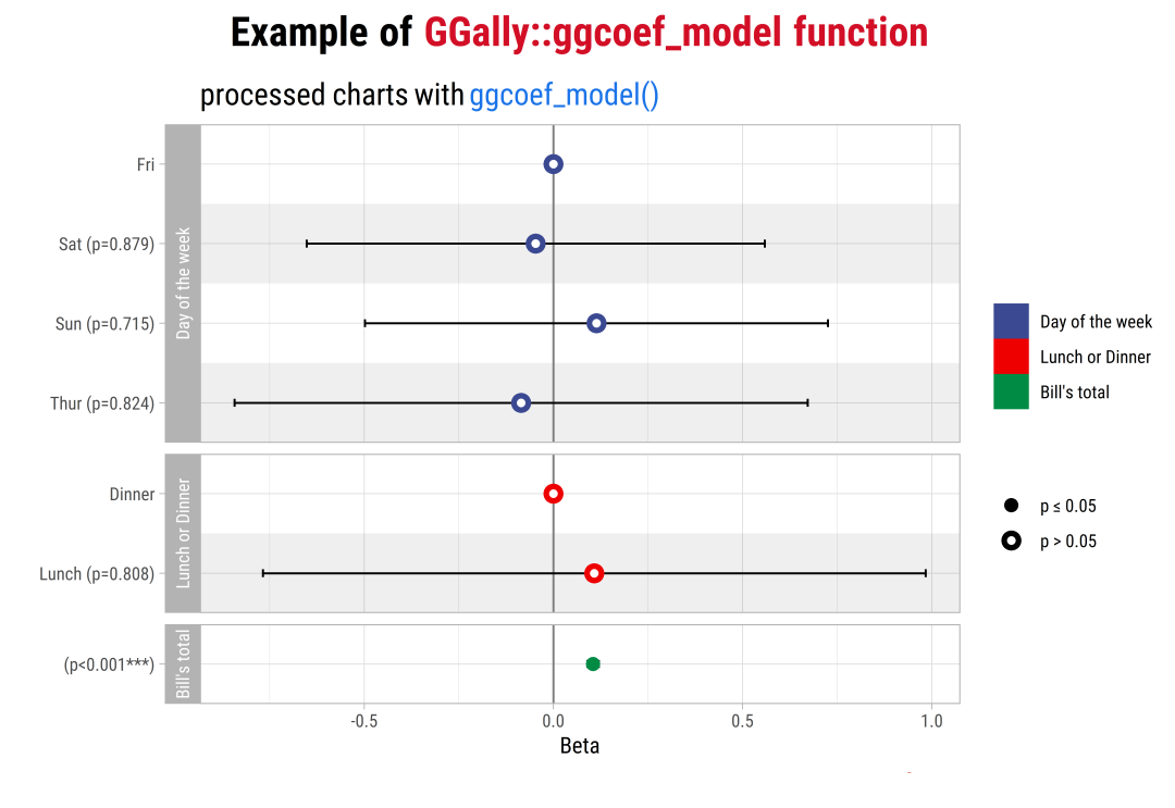
Example of ggcoef_model()

绘图技巧 | 快速绘制矩阵可视化统计图表技巧

R-GGally包简介

官网

主要绘图函数简介

R-GGally包主要函数示例

ggmatrix()绘图函数

ggpairs()绘图函数

ggally_*系列

ggally_cross()

ggally_densityDiag()

ggbivariate()绘图函数

ggnostic()绘图函数