习题6.2

习题6.2

  写出Logistic回归模型学习的梯度下降算法。

解答：

对于Logistic模型：

对数似然函数为：

似然函数求偏导，可得

梯度函数为：

Logistic回归模型学习的梯度下降算法：
(1) 取初始值，置 k=0
(2) 计算
(3) 计算梯度，当时，停止迭代，令；否则，求，使得
(4) 置，计算，当或时，停止迭代，令
(5) 否则，置 k=k+1，转(3)

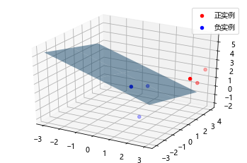
%matplotlib inline
import numpy as np
import time
import matplotlib.pyplot as plt
from mpl_toolkits.mplot3d import Axes3D
from pylab import mpl
# 图像显示中文
mpl.rcParams['font.sans-serif'] = ['Microsoft YaHei']
class LogisticRegression:
    def __init__(self, learn_rate=0.1, max_iter=10000, tol=1e-2):
        self.learn_rate = learn_rate  # 学习率
        self.max_iter = max_iter  # 迭代次数
        self.tol = tol  # 迭代停止阈值
        self.w = None  # 权重
    def preprocessing(self, X):
        """将原始X末尾加上一列，该列数值全部为1"""
        row = X.shape[0]
        y = np.ones(row).reshape(row, 1)
        X_prepro = np.hstack((X, y))
        return X_prepro
    def sigmod(self, x):
        return 1 / (1 + np.exp(-x))
    def fit(self, X_train, y_train):
        X = self.preprocessing(X_train)
        y = y_train.T
        # 初始化权重w
        self.w = np.array([[0] * X.shape[1]], dtype=np.float)
        k = 0
        for loop in range(self.max_iter):
            # 计算梯度
            z = np.dot(X, self.w.T)
            grad = X * (y - self.sigmod(z))
            grad = grad.sum(axis=0)
            # 利用梯度的绝对值作为迭代中止的条件
            if (np.abs(grad) <= self.tol).all():
                break
            else:
                # 更新权重w 梯度上升——求极大值
                self.w += self.learn_rate * grad
                k += 1
        print("迭代次数：{}次".format(k))
        print("最终梯度：{}".format(grad))
        print("最终权重：{}".format(self.w[0]))
    def predict(self, x):
        p = self.sigmod(np.dot(self.preprocessing(x), self.w.T))
        print("Y=1的概率被估计为：{:.2%}".format(p[0][0]))  # 调用score时，注释掉
        p[np.where(p > 0.5)] = 1
        p[np.where(p < 0.5)] = 0
        return p
    def score(self, X, y):
        y_c = self.predict(X)
        error_rate = np.sum(np.abs(y_c - y.T)) / y_c.shape[0]
        return 1 - error_rate
    def draw(self, X, y):
        # 分离正负实例点
        y = y[0]
        X_po = X[np.where(y == 1)]
        X_ne = X[np.where(y == 0)]
        # 绘制数据集散点图
        ax = plt.axes(projection='3d')
        x_1 = X_po[0, :]
        y_1 = X_po[1, :]
        z_1 = X_po[2, :]
        x_2 = X_ne[0, :]
        y_2 = X_ne[1, :]
        z_2 = X_ne[2, :]
        ax.scatter(x_1, y_1, z_1, c="r", label="正实例")
        ax.scatter(x_2, y_2, z_2, c="b", label="负实例")
        ax.legend(loc='best')
        # 绘制p=0.5的区分平面
        x = np.linspace(-3, 3, 3)
        y = np.linspace(-3, 3, 3)
        x_3, y_3 = np.meshgrid(x, y)
        a, b, c, d = self.w[0]
        z_3 = -(a * x_3 + b * y_3 + d) / c
        ax.plot_surface(x_3, y_3, z_3, alpha=0.5)  # 调节透明度
        plt.show()
# 训练数据集
X_train = np.array([[3, 3, 3], [4, 3, 2], [2, 1, 2], [1, 1, 1], [-1, 0, 1],[2, -2, 1]])
y_train = np.array([[1, 1, 1, 0, 0, 0]])
# 构建实例，进行训练
clf = LogisticRegression()
clf.fit(X_train, y_train)
clf.draw(X_train, y_train)
迭代次数：3232次
最终梯度：[ 0.00144779  0.00046133  0.00490279 -0.00999848]
最终权重：[  2.96908597   1.60115396   5.04477438 -13.43744079]

**