参照图3.1,在二维空间中给出实例点,画出k为1和2时的k近邻法构成的空间划分,并对其进行比较,体会k值选择与模型复杂度及预测准确率的关系。
解:
import numpy as npimport matplotlib.pyplot as pltfrom matplotlib.colors import ListedColormapfrom sklearn.neighbors import KNeighborsClassifier# 实例点x = np.array([[0.5, 0.9], [0.7, 2.8], [1.3, 4.6], [1.4, 2.8], [1.7, 0.8], [1.9, 1.4], [2, 4], [2.3, 3], [2.5, 2.5], [2.9, 2],[2.9, 3], [3, 4.5], [3.3, 1.1], [4, 3.7], [4, 2.2], [4.5, 2.5], [4.6, 1], [5, 4]])# 类别y = np.array([0, 1, 0, 1, 1, 1, 0, 0, 1, 0, 0, 0, 1, 0, 0, 0, 1, 0])# 设置二维网格的边界x_min, x_max = 0, 6y_min, y_max = 0, 6# 设置不同类别区域的颜色cmap_light = ListedColormap(['#FFFFFF', '#BDBDBD'])# 生成二维网格h = .01xx, yy = np.meshgrid(np.arange(x_min, x_max, h), np.arange(y_min, y_max, h))# 这里的参数n_neighbors就是k近邻法中的kknn = KNeighborsClassifier(n_neighbors=2)knn.fit(x, y)# ravel()实现扁平化,比如将形状为3*4的数组变成1*12# np.c_()在列方向上连接数组,要求被连接数组的行数相同Z = knn.predict(np.c_[xx.ravel(), yy.ravel()])Z = Z.reshape(xx.shape)plt.figure()# 设置坐标轴的刻度plt.xticks(tuple([x for x in range(6)]))plt.yticks(tuple([y for y in range(6) if y != 0]))# 填充不同分类区域的颜色plt.pcolormesh(xx, yy, Z, cmap=cmap_light)# 设置坐标轴标签plt.xlabel('$x^{(1)}$')plt.ylabel('$x^{(2)}$')# 绘制实例点的散点图plt.scatter(x[:, 0], x[:, 1], c=y)plt.show()
k=1时的KNN算法构成的空间划分: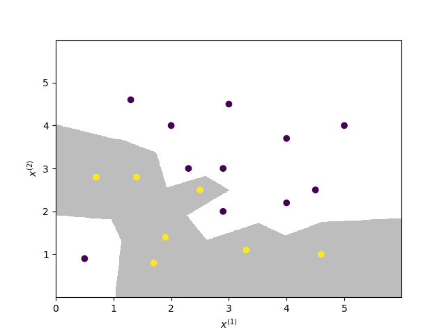
k=2时的KNN算法构成的空间划分: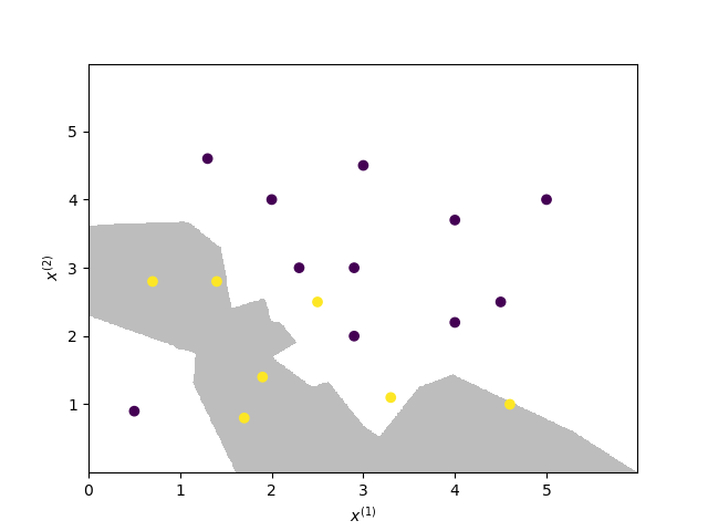

若有收获,就点个赞吧
0 人点赞
