signature 生存分析复现

陷入怀疑😓

signature 生存分析复现

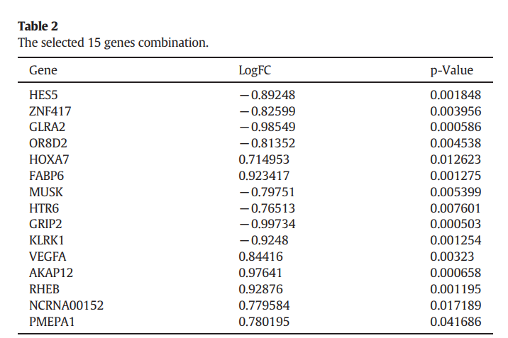
Xu G, Zhang M, Zhu H, et al. A 15-gene signature for prediction of colon cancer recurrence and prognosis based on SVM[J]. Gene, 2017, 604: 33-40.

identify signature

library(GEOquery)
library(AnnotationDbi)
library(org.Hs.eg.db)

DEG

GSE17537（以这个数据集为基础找差异表达基因）

data in GSE17537 were analyzed using the Linear Models for Microarray data (LIMMA) method to identify the differentially expressed genes (DEGs). Preprocessed data were normalized by Z-score transformation… The threshold for identification of DEGs was set as p < 0.05 and |logFC(fold change)| > 0.7.

f <- 'GSE17537.Rdata'
if(!file.exists(f)){
  gset <- getGEO('GSE17537',destdir = '.',
                 AnnotGPL = F,
                 getGPL = F)
  save(gset,file=f)
}
load('GSE17537.Rdata')
degexpr <- exprs(gset[[1]])
degpdat <- pData(gset[[1]])
degexpr[1:4,1:4]
#           GSM437270 GSM437271 GSM437272 GSM437273
# 1007_s_at 10.636083 11.042240 11.015748 10.734469
# 1053_at    7.974253  8.542731  7.190542  8.731533
# 117_at     8.242136  7.271520  7.368352  7.027436
# 121_at     9.315796  9.277670  9.325623  9.398863
## z-score
degexpr <- t(scale(t(degexpr)))
degexpr[1:4,1:4]
#            GSM437270  GSM437271  GSM437272  GSM437273
# 1007_s_at -0.6468308  0.4474904  0.3761127 -0.3817476
# 1053_at   -0.6561249  0.3432638 -2.0338972  0.6751799
# 117_at     1.8993885  0.1023676  0.2816449 -0.3495356
# 121_at    -1.0241496 -1.2322858 -0.9705000 -0.5706729
degsymb <- select(hgu133plus2.db,row.names(degexpr),"SYMBOL","PROBEID")
degtrim <- degsymb[match(unique(degsymb$SYMBOL),degsymb$SYMBOL),]
degtrim <- na.omit(degtrim)
degexpr <-  degexpr[degtrim$PROBEID,]
row.names(degexpr) <- degtrim$SYMBOL
dim(degexpr)
# [1] 1399   55
save(degexpr, file = "GEO-degexpr.Rdata")
save(degpdat,file = "GEO-degpdat.Rdata")

DEG筛选

rm(list = ls())
load("GEO-degexpr.Rdata")
load("GEO-degpdat.Rdata")
library(limma)
table(degpdat$`dfs_event (disease free survival; cancer recurrence):ch1`)
# 
# no recurrence    recurrence 
#            36            19 
group_list <- degpdat$`dfs_event (disease free survival; cancer recurrence):ch1`
design <- model.matrix(~0+factor(group_list))
colnames(design) <- c("no", "re")
rownames(design) <- colnames(degexpr)
contrast.matrix <- makeContrasts('no-re',levels = design) 
fit <- lmFit(degexpr, design)
fit1 <- contrasts.fit(fit, contrast.matrix) 
fit2 <- eBayes(fit1)
DEGstb <- topTable(fit2, coef=1, n=Inf)
DEGmtx <- na.omit(DEGstb)
DEGmtx <- DEGmtx[absDEGmtx$logFC]
DEGmtx$result <- ifelse(DEGmtx$P.Value < 0.05 &
                       abs(DEGmtx$logFC) > 0.7,
                     ifelse(DEGmtx$logFC > 0.7,
                            "UP", "DOWN"), "NOT")
table(DEGmtx$result)
# 
# DOWN  NOT   UP 
#   14 1314   71 
head(DEGmtx)
#              logFC       AveExpr        t      P.Value adj.P.Val          B result
# DDX31    1.1059228  2.267284e-15 3.931463 8.450714e-05 0.1182255  0.8853818     UP
# C11orf42 0.9940823 -5.083371e-16 3.533879 4.097569e-04 0.1661362 -0.3317710     UP
# ACACB    0.9625943  3.113513e-15 3.421942 6.220910e-04 0.1661362 -0.6510647     UP
# PGLS     0.9068060 -8.080973e-16 3.223619 1.266363e-03 0.1661362 -1.1915345     UP
# STARD6   0.9032174 -1.506371e-16 3.210862 1.323938e-03 0.1661362 -1.2251955     UP
# IRAK2    0.8952166  4.313153e-16 3.182420 1.461101e-03 0.1661362 -1.2997641     UP

文献中的DEG筛选结果：

A total of 1207 genes were identified as DEGs between recurrence and no-recurrence samples, including 726 downregulated and 481 upregulated genes.

我的筛选结果：

table(DEGmtx$result)
# 
# DOWN  NOT   UP 
#   14 1314   71
save(DEGmtx, file = "DEGs.Rdata")

signature

To obtain the optimal feature genes for diagnosing recurrence, SVM-RFE algorithm was performed using genes as features and their expression levels as feature values. As a result, 85% prediction accuracy was found to be achieved using a 15-gene combination.

这一步应该在我浅薄的能力之外…

直接在前面得到的DEG中找这15个基因：

paper_signature <- DEGmtx[c("HES5","ZNF417","GLRA2","OR8D2","HOXA7","FABP6",
                          "MUSK","HTR6","GRIP2","KLRK1","VEGFA","AKAP12","RHEB",
                          "NCRNA00152","PMEPA1"),]

基因 signature 生存分析复现 - 图2

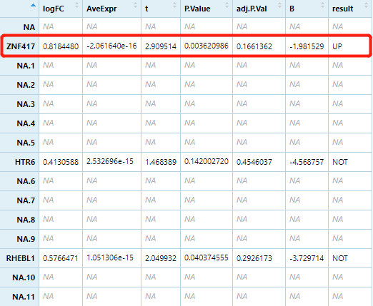
但只有3个基因在筛选的DEG/下载的表达矩阵中，只有 ZNF417 为差异表达基因。

鉴于并不知道怎么得到signature….依然只能直接进行文章中的 Validation analysis

数据准备

GEO

GSE38832

if(!file.exists(f)){
  gset <- getGEO('GSE38832',destdir = '.',
                 AnnotGPL = F,
                 getGPL = F)
  save(gset,file=f)
}
load('GSE38832.Rdata')
expr1 <- exprs(gset[[1]])
pdat1 <- pData(gset[[1]])
expr1[1:4,1:4]
#           GSM950411 GSM950412 GSM950413 GSM950414
# 1007_s_at 12.015001 12.319230 12.268841 12.309278
# 1053_at    9.600642  9.991989  9.349406  8.934902
# 117_at     8.125449  7.661441 11.611829  8.575235
# 121_at    10.868107 11.191637 10.794642 11.157243
expr1 <- log2(expr1+1)
symb1 <- select(hgu133plus2.db,row.names(expr1),"SYMBOL","PROBEID")
trim1 <- symb1[match(unique(symb1$SYMBOL),symb1$SYMBOL),]
trim1 <- na.omit(trim1)
expr1 <-  expr1[trim1$PROBEID,]
row.names(expr1) <- trim1$SYMBOL
save(expr1, file = "GEO-expr1.Rdata")

GSE17538

只有6个样本，并非文献中的200多个，ID转换过程中发现下载到的是小鼠…?

去官网直接下载，发现好像失效了，无法下载——弃。

基因 signature 生存分析复现 - 图3

f <- 'GSE17538.Rdata'
if(!file.exists(f)){
  gset <- getGEO('GSE17538',destdir = '.',
                 AnnotGPL = F,
                 getGPL = F)
  save(gset,file=f)
}
load('GSE17538.Rdata')
expr2 <- exprs(gset[[1]])
pdat2 <- pData(gset[[1]])
expr2[1:4,1:4]
#            GSM472198 GSM472199 GSM472200 GSM472201
# 1415670_at  9.284539  9.239952  9.311207  9.501534
# 1415671_at 10.668639 10.677101 10.637565 10.872466
# 1415672_at 10.624298 10.563723 10.540626 10.685249
# 1415673_at 10.323815 10.267230 10.453991  9.791176
expr2 <- log2(expr2+1)
BiocManager::install("mouse4302.db")
library(mouse4302.db)
symb2 <- select(mouse4302.db,row.names(expr2),"SYMBOL","PROBEID")
trim2 <- symb2[match(unique(symb2$SYMBOL),symb2$SYMBOL),]
trim2 <- na.omit(trim2)
expr2 <-  expr2[trim2$PROBEID,]
row.names(expr2) <- trim2$SYMBOL
save(expr2, file = "GEO-expr2.Rdata")

GSE28814

基因 signature 生存分析复现 - 图4

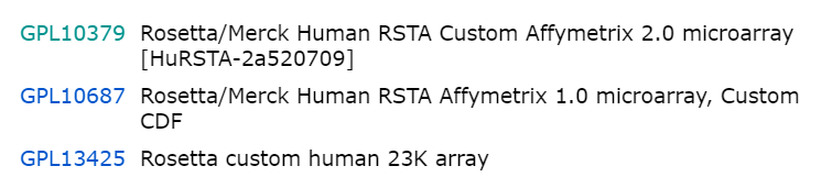
没有找到对应的注释R包，从 GPL10379 Rosetta/Merck Human RSTA Custom Affymetrix 2.0 microarray [HuRSTA-2a520709] Data table 手动导出txt。

需要在excel中打开调整分隔符重新保存，才能在R中正确读取。

f <- 'GSE28814.Rdata'
if(!file.exists(f)){
  gset <- getGEO('GSE28814',destdir = '.',
                 AnnotGPL = F,
                 getGPL = F)
  save(gset,file=f)
}
load('GSE28814.Rdata')
expr3 <- exprs(gset[[1]])
pdat3 <- pData(gset[[1]])
expr3[1:4,1:4]
#                  GSM707237 GSM707238 GSM707239 GSM707240
# 100121619_TGI_at 2.4105105 1.9840042 2.9346733 2.4020889
# 100121620_TGI_at 2.3519606 2.1129721 2.0588146 1.6712892
# 100121621_TGI_at 1.2706607 0.7851753 1.4145823 1.5996047
# 100121622_TGI_at 0.8892922 1.0277808 0.6097267 0.7636354
anno <- read.table('./HuRSTA-2a520709.txt',sep = "\t",header = T,
                   na.strings = NA, stringsAsFactors = F)
anno[1:4,1:4]
#                 ID EntrezGeneID GeneSymbol    GB_ACC
# 1 100138926_TGI_at         6566    SLC16A1  BC026317
# 2 100131045_TGI_at           NA             BX098869
# 3 100134882_TGI_at         3458       IFNG NM_000619
#  4 100149534_TGI_at        51552      RAB14  AK090889

TCGA

GDC TCGA Colon Cancer (COAD) TCGA Colon Cancer (COAD)&removeHub=https%3A%2F%2Fxena.treehouse.gi.ucsc.edu%3A443) (15 datasets)
- HTSeq - Counts (n=512) GDC Hub
- Phenotype (n=571) GDC Hub
- survival data (n=539) GDC Hub

expr4 <- read.table('./TCGA-COAD.htseq_counts.tsv/TCGA-COAD.htseq_counts.tsv',header = T,sep='\t')
tail(expr4[,1])
# [1] ENSGR0000281849.1      __no_feature           __ambiguous           
# [4] __too_low_aQual        __not_aligned          __alignment_not_unique
# 60488 Levels: __alignment_not_unique __ambiguous __no_feature __not_aligned ... ENSGR0000281849.1
class(expr4[,1])
# [1] "factor"
expr4[,1] <- as.character(expr4[,1])
for (i in 1:nrow(expr4)) {
  expr4[i,1] <- strsplit(expr4[i,1],"\\.")[[1]][1]
}
row.names(expr4) <- expr4[,1]
expr4 <- expr4[,-1]
symb4 <- select(org.Hs.eg.db,expr4[,1],"SYMBOL","ENSEMBL")
trim4 <- symb4[match(unique(symb4$SYMBOL),symb4$SYMBOL),]
trim4 <- na.omit(trim4)
expr4 <-  expr4[trim4$ENSEMBL,]
row.names(expr4) <- trim4$SYMBOL
expr4[1:4,1:4]
#        TCGA.DM.A288.01A TCGA.QL.A97D.01A TCGA.CM.6164.01A TCGA.G4.6299.01A
# TSPAN6        10.985842        12.391512        13.857787         9.807355
# TNMD           3.700440         7.531381         6.714246         1.000000
# DPM1          11.163650        11.798472        12.496354        11.004220
# SCYL3          9.262095         9.581201         9.419960         9.903882
expr4 <- log2(expr4+1)
save(expr4, file = "TCGA-expr.Rdata")

Validation analysis

GSE38832

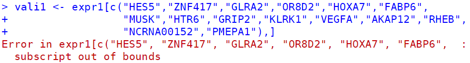
vali1 <- expr1[c("HES5","ZNF417","GLRA2","OR8D2","HOXA7","FABP6",
                 "MUSK","HTR6","GRIP2","KLRK1","VEGFA","AKAP12","RHEB",
                 "NCRNA00152","PMEPA1"),]

基因 signature 生存分析复现 - 图5

GSE28814

vali3 <- expr3[c("HES5","ZNF417","GLRA2","OR8D2","HOXA7","FABP6",
                 "MUSK","HTR6","GRIP2","KLRK1","VEGFA","AKAP12","RHEB",
                 "NCRNA00152","PMEPA1"),]

基因 signature 生存分析复现 - 图6

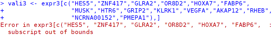
结果居然一个都没有….

TCGA

vali4 <- expr4[c("HES5","ZNF417","GLRA2","OR8D2","HOXA7","FABP6",
                 "MUSK","HTR6","GRIP2","KLRK1","VEGFA","AKAP12","RHEB",
                 "NCRNA00152","PMEPA1"),]
row.names(vali4)
#  [1] "HES5"   "ZNF417" "GLRA2"  "OR8D2"  "HOXA7"  "FABP6"  "MUSK"   "HTR6"   "GRIP2" 
# [10] "KLRK1"  "VEGFA"  "AKAP12" "RHEB"   "NA"     "PMEPA1"

缺少 NCRNA00152

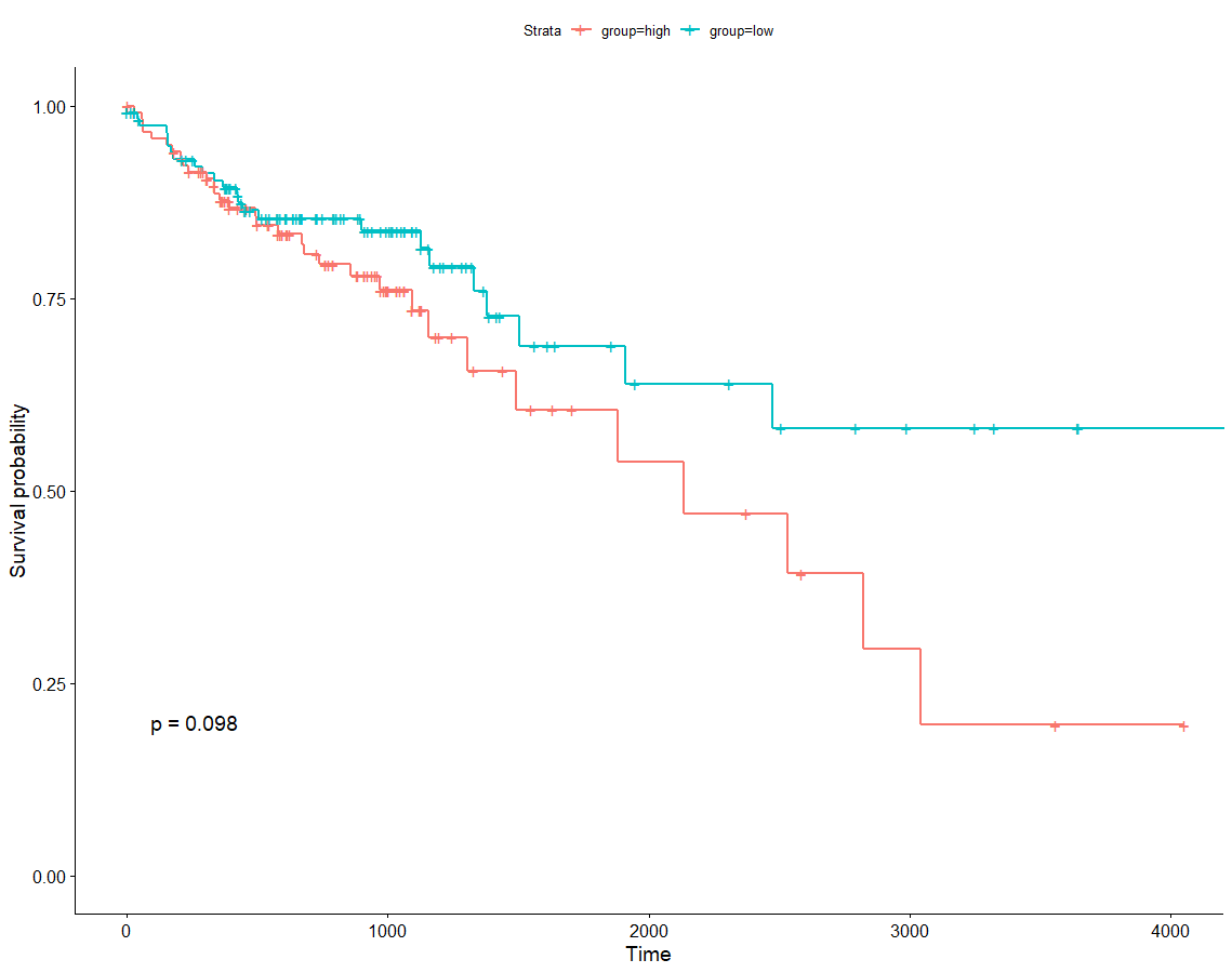
KM plot (TCGA data)

vali4 <- expr4[c("HES5","ZNF417","GLRA2","OR8D2","HOXA7","FABP6",
                 "MUSK","HTR6","GRIP2","KLRK1","VEGFA","AKAP12","RHEB",
                 "NCRNA00152","PMEPA1"),]
row.names(vali4)
vali4 <- na.omit(vali4)
clin$submitter_id.samples = gsub('-','.',clin$submitter_id.samples)
row.names(clin) <- clin[,1]
#### 筛选复发病人，并无有用信息
table(clin$progression_or_recurrence.diagnoses)
# 
#              not reported 
#            2          268 
surv$sample <- gsub('-','.',surv$sample)
row.names(surv) <- surv[,1]
surv <- surv[surv$sample %in% row.names(clin),]
clin <- clin[row.names(clin) %in% surv$sample,]
phe <- cbind(clin,surv[,c("OS.time","OS")])
vali4 <- vali4[,colnames(vali4) %in% row.names(phe)]
phe <- phe[row.names(phe) %in% colnames(vali4),]
dim(phe)
vali4 <- as.matrix(vali4)
#### 将14个基因视为一个对象
for(i in 1:ncol(vali4)){
   sig[i] <- sum(vali4[,i])
 }
group <- ifelse(sig > median(sig),'high','low') 
phe$group <- group
phe <- phe[,c("OS.time","OS","group")]
ggsurvplot(survfit(Surv(OS.time, OS)~group, data=phe), pval=TRUE)

基因 signature 生存分析复现 - 图7

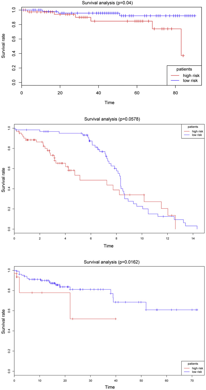
文章中是这样的：

The results indicated that patients with different recurrent risks could exhibit a significantly different

prognosis in two datasets: GSE38832, p = 0.04, Fig. 5A; GSE28814, p = 0.0578, Fig. 5B; and TCGA, p = 0.0162, Fig. 5C.