Liu G, Zeng X, Wu B, et al. RNA-Seq analysis of peripheral blood mononuclear cells reveals unique transcriptional signatures associated with radiotherapy response of nasopharyngeal carcinoma and prognosis of head and neck cancer[J]. Cancer biology & therapy, 2020, 21(2): 139-146.
四种方法p值对比
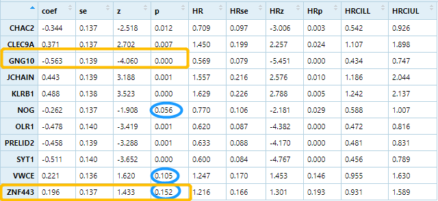
| Cox | median | km | best cut | |
|---|---|---|---|---|
| GNG10 | <0.0001 | 0.00044 | 0.00055 | 0.00018 |
| ZNF443 | 0.152 | 0.1 | 0.54 | 0.02 |
取上次分析 p 值最小/最大的两个基因:
rm(list = ls())options(stringsAsFactors = F)load(file='../HNSC_expr.Rdata')exprSet=exprdatExpr=log2(edgeR::cpm(exprSet)+1)load("../HNSC_phe.Rdata")dat <- phedat$GNG10=c(t(datExpr['GNG10',]))dat$ZNF443=c(t(datExpr['ZNF443',]))head(dat)# race age stage radiation time event GNG10# TCGA.BB.4224.01A white 52 Stage III YES 278 0 5.611493# TCGA.H7.7774.01A white 75 Stage III YES 407 0 5.823435# TCGA.CV.6943.01A white 74 Stage III 602 1 5.759393# TCGA.CN.5374.01A white 56 Stage IVA YES 1732 1 5.685456# TCGA.CQ.6227.01A white 77 Stage III NO 129 1 5.759871# TCGA.CV.6959.01A white 48 Stage III NO 256 1 5.767435# ZNF443# TCGA.BB.4224.01A 5.611675# TCGA.H7.7774.01A 5.690211# TCGA.CV.6943.01A 5.663535# TCGA.CN.5374.01A 5.660077# TCGA.CQ.6227.01A 5.530966# TCGA.CV.6959.01A 5.661470
1 median method
library(survival)library("survminer")library(ggplot2)
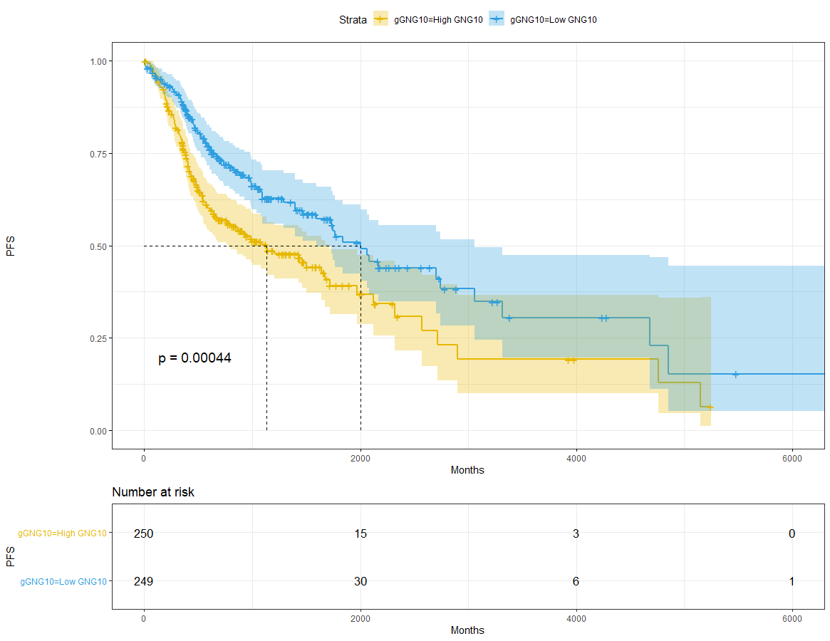
GNG10
dat$gGNG10=ifelse(dat$GNG10<median(dat$GNG10),'Low GNG10','High GNG10')sfit_GNG10 = survfit(Surv(time,event) ~ gGNG10, data = dat)sfit_GNG10# Call: survfit(formula = Surv(time, event) ~ gGNG10, data = dat)## 1 observation deleted due to missingness# n events median 0.95LCL 0.95UCL# gGNG10=High GNG10 250 125 1133 773 1718# gGNG10=Low GNG10 249 93 2002 1591 3059ggsurvplot(sfit_GNG10,pval = T,conf.int = T,risk.table = T,surv.median.line = 'hv',ggtheme = theme_bw(),palette = c('#E7B800','#2E9FDF'))+xlab('Months') + ylab('PFS')
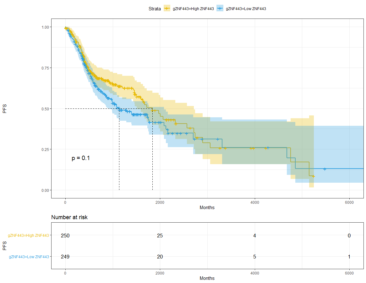
ZNF443
dat$gZNF443=ifelse(dat$ZNF443<median(dat$ZNF443),'Low ZNF443','High ZNF443')sfit_ZNF443 = survfit(Surv(time,event) ~ gZNF443, data = dat)sfit_ZNF443# Call: survfit(formula = Surv(time, event) ~ gZNF443, data = dat)## 1 observation deleted due to missingness# n events median 0.95LCL 0.95UCL# gZNF443=High ZNF443 250 97 1838 1504 2717# gZNF443=Low ZNF443 249 121 1133 927 2083ggsurvplot(sfit_ZNF443,pval = T,conf.int = T,risk.table = T,surv.median.line = 'hv',ggtheme = theme_bw(),palette = c('#E7B800','#2E9FDF'))+xlab('Months') + ylab('PFS')
2 survivalROC package, km method
其实没太搞明白 predict.time 的设置原则
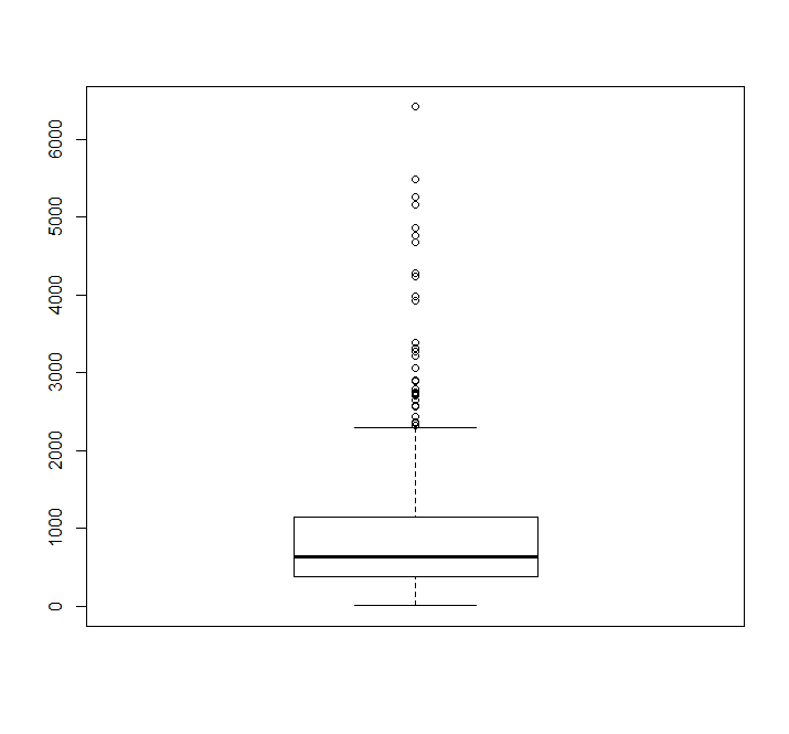
boxplot(dat$time)library(survivalROC)cuttime=1000 ## 暂且设为1000
GNG10
sroc=survivalROC(Stime = dat$time,status = dat$event,marker = dat$GNG10,predict.time = cuttime,method = 'KM')cut.op=sroc$cut.values[which.max(sroc$TP-sroc$FP)]cut.op# [1] 5.762685
plot(sroc$FP,sroc$TP,type = 'l',xlim = c(0,1),ylim = c(0,1),xlab = paste('FP','\n','AUC=',round(sroc$AUC,3)),ylab = 'TP',main = 'survival ROC',col='red')abline(0,1)legend('bottomright',c('gene expression'),col = 'red',lty = c(1,1))
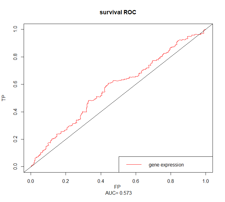
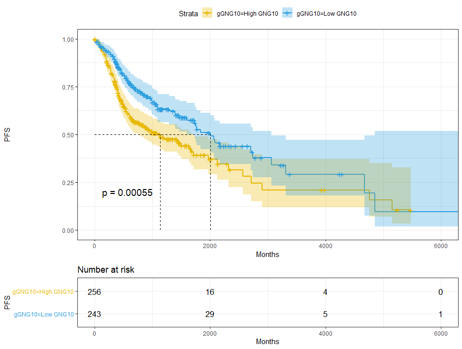
dat$gGNG10=ifelse(dat$GNG10 < cut.op,'Low GNG10','High GNG10')sfit = survfit(Surv(time,event) ~ gGNG10, data = dat)sfit# Call: survfit(formula = Surv(time, event) ~ gGNG10, data = dat)## 1 observation deleted due to missingness# n events median 0.95LCL 0.95UCL# gGNG10=High GNG10 256 128 1133 763 1718# gGNG10=Low GNG10 243 90 2002 1591 3059ggsurvplot(sfit,pval = T,conf.int = T,risk.table = T,surv.median.line = 'hv',ggtheme = theme_bw(),palette = c('#E7B800','#2E9FDF'))+xlab('Months') + ylab('PFS')
ZNF443
cuttime=1000sroc=survivalROC(Stime = dat$time,status = dat$event,marker = dat$ZNF443,predict.time = cuttime,method = 'KM')cut.op=sroc$cut.values[which.max(sroc$TP-sroc$FP)]cut.op# [1] 5.747971
plot(sroc$FP,sroc$TP,type = 'l',xlim = c(0,1),ylim = c(0,1),xlab = paste('FP','\n','AUC=',round(sroc$AUC,3)),ylab = 'TP',main = 'survival ROC',col='red')abline(0,1)legend('bottomright',c('gene expression'),col = 'red',lty = c(1,1))
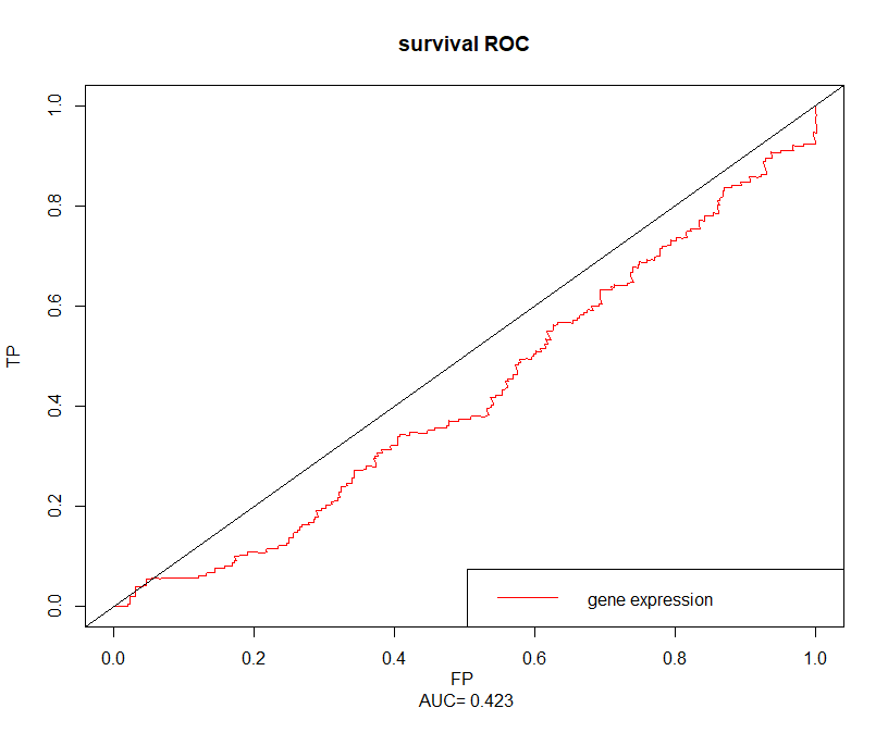
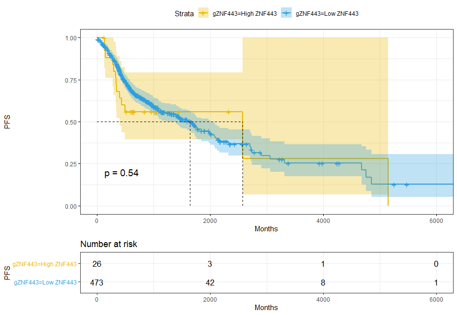
dat$gZNF443=ifelse(dat$ZNF443 < cut.op,'Low ZNF443','High ZNF443')sfit = survfit(Surv(time,event) ~ gZNF443, data = dat)sfit# Call: survfit(formula = Surv(time, event) ~ gZNF443, data = dat)## 1 observation deleted due to missingness# n events median 0.95LCL 0.95UCL# gZNF443=High ZNF443 26 13 2570 395 NA# gZNF443=Low ZNF443 473 205 1641 1289 2002ggsurvplot(sfit,pval = T,conf.int = T,risk.table = T,surv.median.line = 'hv',ggtheme = theme_bw(),palette = c('#E7B800','#2E9FDF'))+xlab('Months') + ylab('PFS')
3 survminer package, find the best surv_cutpoint
cut_point=surv_cutpoint(dat,time = 'time',event = 'event',variables = c('GNG10','ZNF443'))summary(cut_point)# cutpoint statistic# GNG10 5.762685 3.735037# ZNF443 5.702524 2.398513res_cat=surv_categorize(cut_point)head(res_cat)# time event GNG10 ZNF443# TCGA.BB.4224.01A 278 0 low low# TCGA.H7.7774.01A 407 0 high low# TCGA.CV.6943.01A 602 1 low low# TCGA.CN.5374.01A 1732 1 low low# TCGA.CQ.6227.01A 129 1 low low# TCGA.CV.6959.01A 256 1 high low
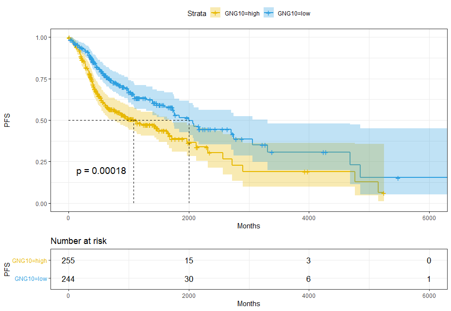
GNG10
sfit = survfit(Surv(time,event) ~ GNG10, data = res_cat)sfit# Call: survfit(formula = Surv(time, event) ~ GNG10, data = res_cat)## 1 observation deleted due to missingness# n events median 0.95LCL 0.95UCL# GNG10=high 255 128 1081 763 1671# GNG10=low 244 90 2002 1732 3314ggsurvplot(sfit,pval = T,conf.int = T,risk.table = T,surv.median.line = 'hv',ggtheme = theme_bw(),palette = c('#E7B800','#2E9FDF'))+xlab('Months') + ylab('PFS')
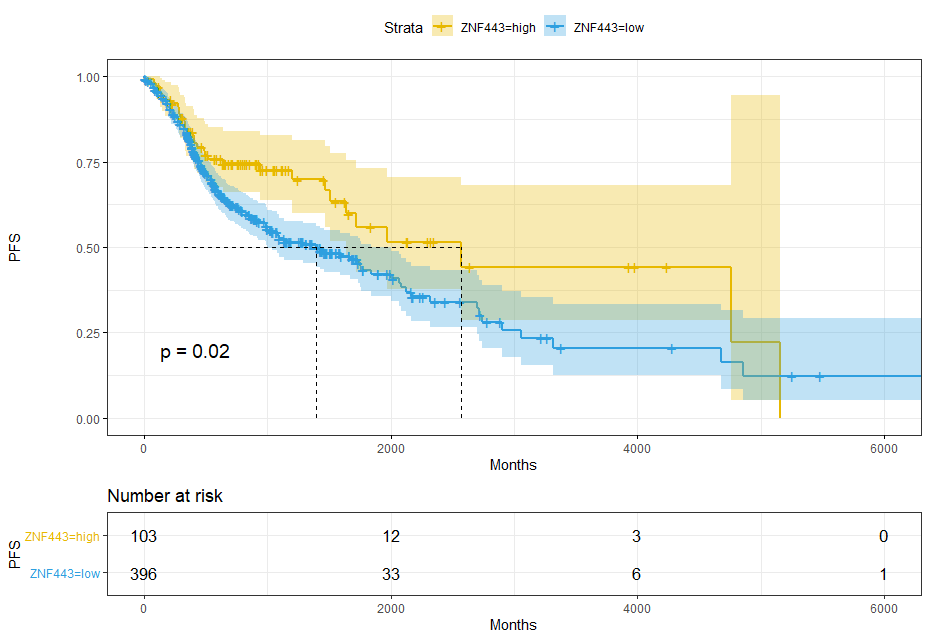
ZNF443
sfit = survfit(Surv(time,event) ~ ZNF443, data = res_cat)sfit# Call: survfit(formula = Surv(time, event) ~ ZNF443, data = res_cat)## 1 observation deleted due to missingness# n events median 0.95LCL 0.95UCL# ZNF443=high 103 34 2570 1641 NA# ZNF443=low 396 184 1398 998 1838ggsurvplot(sfit,pval = T,conf.int = T,risk.table = T,surv.median.line = 'hv',ggtheme = theme_bw(),palette = c('#E7B800','#2E9FDF'))+xlab('Months') + ylab('PFS')

若有收获,就点个赞吧
0 人点赞
