YTHDF1在卵巢癌的预后

1. 数据准备

下载

[cohort: GDC TCGA Ovarian Cancer (OV)]

• HTSeq - Counts (n=379) GDC Hub
• Phenotype (n=758) GDC Hub
• survival data (n=731) GDC Hub

读入/整合

library(AnnotationDbi)
library(org.Hs.eg.db)
library(survival)
library(survminer)

• 表达矩阵

expr <- read.table('./TCGA-OV.htseq_counts.tsv/TCGA-OV.htseq_counts.tsv',header = T,sep='\t')
  dim(expr)
# [1] 60488   380
expr[1:4,1:4]
#           Ensembl_ID TCGA.23.1120.01A TCGA.29.1695.01A TCGA.61.2003.01A
# 1 ENSG00000000003.13        12.308908        12.298063         11.34430
# 2  ENSG00000000005.5         3.000000         3.906891          1.00000
# 3 ENSG00000000419.11        11.587309        11.433585         11.84549
# 4 ENSG00000000457.12         9.147205        10.601771         10.23122
tail(expr[,1])
# [1] "ENSGR0000281849.1"      "__no_feature"           "__ambiguous"           
# [4] "__too_low_aQual"        "__not_aligned"          "__alignment_not_unique"
expr <- expr[1:(nrow(expr)-5),]
class(expr[,1])
# [1] "factor"
expr[,1] <- as.character(expr[,1])
for (i in 1:nrow(expr)) {
  expr[i,1] <- strsplit(expr[i,1],"\\.")[[1]][1]
}
symb <- select(org.Hs.eg.db,expr[,1],"SYMBOL","ENSEMBL")
table(symb[,2]=="YTHDF1")
# 
# FALSE  TRUE 
# 25590     1 
which(symb$SYMBOL=="YTHDF1")
# [1] 9300
thegene <- symb[9300,]
thegene <- expr[expr$Ensembl_ID==thegene$ENSEMBL,]
thegene <- thegene[,-1]
row.names(thegene) <- "YTHDF1"
thegene <- round(thegene,digits = 2)
save(thegene,file='YTHDF1expression.Rdata')

• 临床数据

clin <- read.table('./TCGA-HNSC.GDC_phenotype.tsv',header = T,sep='\t')
summary(clin)
clin[1:4,1:4]
clin$submitter_id.samples = gsub('-','.',clin$submitter_id.samples)
row.names(clin) <- clin[,1]
clin <- clin[c("age_at_initial_pathologic_diagnosis","clinical_stage","person_neoplasm_cancer_status",
               "radiation_therapy","race.demographic")]
colnames(clin) <- c("age","stage","status","radiation","race")
clin <- na.omit(clin)
save(clin,file='clinical.Rdata')

• 生存数据

surv <- read.table('./TCGA-OV.survival.tsv/TCGA-OV.survival.tsv',header = T,sep='\t')

• 整合数据（挑选病人)

surv$sample <- gsub('-','.',surv$sample)
row.names(surv) <- surv[,1]
surv <- surv[surv$sample %in% row.names(clin),]
clin <- clin[row.names(clin) %in% surv$sample,]
phe <- cbind(clin,surv[,c("OS.time","OS")])
thegene <- thegene[,colnames(thegene) %in% row.names(phe)]
phe <- phe[row.names(phe) %in% colnames(thegene),]
# table(row.names(phe) %in% colnames(thegene))
dim(phe)
# [1] 188   7
save(phe,file='phe_surv.Rdata')

2. cox

mySurv=with(phe,Surv(OS.time, OS))

univariate cox regression

unicox <-apply(thegene, 1 ,function(gene){
  group=ifelse(gene>median(gene),'high','low') 
  survival_dat <- data.frame(group=group,stage=phe$stage,age=phe$age,status=phe$status,
                             radiation=phe$radiation,race=phe$race,stringsAsFactors = F)
  m=coxph(mySurv ~group, data =  survival_dat)
  beta <- coef(m)
  se <- sqrt(diag(vcov(m)))
  HR <- exp(beta)
  HRse <- HR * se
  tmp <- round(cbind(coef = beta, se = se, z = beta/se, p = 1 - pchisq((beta/se)^2, 1),
                     HR = HR, HRse = HRse,
                     HRz = (HR - 1) / HRse, HRp = 1 - pchisq(((HR - 1)/HRse)^2, 1),
                     HRCILL = exp(beta - qnorm(.975, 0, 1) * se),
                     HRCIUL = exp(beta + qnorm(.975, 0, 1) * se)), 3)
  return(tmp['grouplow',])
})
unicox=t(unicox)
table(unicox[,4]<0.05)
# 
# FALSE 
#     1 
unicox[,4]
# [1] 0.933

multivariate cox regression

multicox <-apply(thegene, 1 ,function(gene){
  group=ifelse(gene>median(gene),'high','low') 
  survival_dat <- data.frame(group=group,stage=phe$stage,age=phe$age,status=phe$status,
                             radiation=phe$radiation,race=phe$race,stringsAsFactors = F)
  m=coxph(mySurv ~   age + stage+ group+status+radiation+race, data =  survival_dat)
  beta <- coef(m)
  se <- sqrt(diag(vcov(m)))
  HR <- exp(beta)
  HRse <- HR * se
  tmp <- round(cbind(coef = beta, se = se, z = beta/se, p = 1 - pchisq((beta/se)^2, 1),
                     HR = HR, HRse = HRse,
                     HRz = (HR - 1) / HRse, HRp = 1 - pchisq(((HR - 1)/HRse)^2, 1),
                     HRCILL = exp(beta - qnorm(.975, 0, 1) * se),
                     HRCIUL = exp(beta + qnorm(.975, 0, 1) * se)), 3)
  return(tmp['grouplow',])
})
multicox=t(multicox)
table(multicox[,4]<0.05)
# 
# FALSE 
#     1 
multicox[,4]
# [1] 0.982

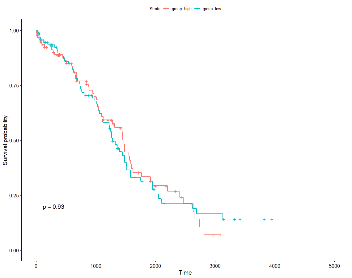
作图

group=ifelse(as.numeric(thegene)>median(as.numeric(thegene)),'high','low') 
phe$group <- group
ggsurvplot(survfit(Surv(OS.time, OS)~group, data=phe), pval=TRUE)