数据下载
UCSC Xena: https://xenabrowser.net/datapages/
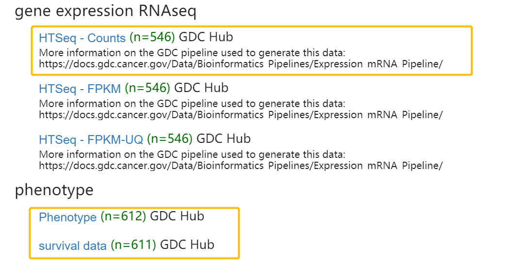
cohort: GDC TCGA Head and Neck Cancer (HNSC)
work with R
1. 读入及初步处理
# 临床数据clin <- read.table('./TCGA-HNSC.GDC_phenotype.tsv',header = T,sep='\t')summary(clin)clin[1:4,1:4]save(clin,file='clinical.Rdata')
# 表达矩阵suppressPackageStartupMessages(library(org.Hs.eg.db))suppressPackageStartupMessages(library(AnnotationDbi))expr <- read.table('./TCGA-HNSC.htseq_counts.tsv',header = T,sep='\t')dim(expr)# [1] 60488 547expr[1:4,1:4]# Ensembl_ID TCGA.BB.4224.01A TCGA.H7.7774.01A TCGA.CV.6943.01A# 1 ENSG00000000003.13 11.127994 11.420487 11.39178# 2 ENSG00000000005.5 1.584963 0.000000 0.00000# 3 ENSG00000000419.11 10.650154 10.724514 10.68825# 4 ENSG00000000457.12 10.055282 9.651052 9.84235enb <- as.character(expr[,1])enb_new <- c()for (i in 1:length(enb)) {enb_new[i] <- strsplit(enb[i],"\\.")[[1]][1]}enb_new <- unique(enb_new)symb <- AnnotationDbi::select(org.Hs.eg.db,enb_new,"SYMBOL","ENSEMBL")todelet <- match(symb[,1],enb_new )expr[,1] <- enb_newexpr <- expr[todelet,]expr[,1] <- symb[,2]gs <- expr$Hugo_Symbolexpr <- expr[,-1]rownames(expr) <- gsexpr <- log2(expr+1)expr <- apply(expr, 2, function(x){as.numeric(format(x,digits = 2))})save(expr,file='expression.Rdata')
clin$submitter_id.samples = gsub('-','.',clin$submitter_id.samples)phe <- clin[match(clin$submitter_id.samples,colnames(expr)),]phe <- phe[is.na(phe[,1]) == FALSE,]
# OSsurv <- read.table('./TCGA-HNSC.survival.tsv',header = T,sep='\t')geneselected <- expr[c("CHAC2","CLEC9A","GNG10","JCHAIN","KLRB1","NOG","OLR1","PRELID2","SYT1","VWCE","ZNF443"),]surv$sample = gsub('-','.',surv$sample)
3. 整合数据
dat <- t(geneselected)OSinfo <- surv[,c("OS.time","OS")]rownames(OSinfo) <- surv$sampledat2 <- dat[row.names(dat) %in% row.names(OSinfo),] %>% na.omit()OSinfo <- OSinfo[row.names(dat2),]dat2 <- cbind(dat2,OSinfo)library(reshape2)dat3 <- melt(dat2,c("OS.time","OS"))colnames(dat3)[3] <- "gene"save(dat3,file = "df_survivalplot.Rdata")
4. cox survival analysis
library(survival)library(survminer)dat3$OS.time <- as.numeric(dat3$OS.time)dat3$group <- ifelse(dat3$value >= 2.8, "High","Low")mySurv_OS <- Surv(dat3$OS.time,dat3$OS)coxfit <- coxph(mySurv_OS ~ gene + group,data = dat3)summary(coxfit)
# Call:# coxph(formula = mySurv_OS ~ gene + group, data = dat3)## n= 5995, number of events= 2772## coef exp(coef) se(coef) z Pr(>|z|)# geneCLEC9A -0.0251926 0.9751221 0.0994572 -0.253 0.800# geneGNG10 0.0008413 1.0008417 0.0890996 0.009 0.992# geneJCHAIN -0.0006175 0.9993826 0.0890938 -0.007 0.994# geneKLRB1 -0.0130832 0.9870020 0.0920338 -0.142 0.887# geneNOG -0.0240868 0.9762010 0.0986196 -0.244 0.807# geneOLR1 -0.0045179 0.9954923 0.0894466 -0.051 0.960# genePRELID2 -0.0024808 0.9975223 0.0891958 -0.028 0.978# geneSYT1 -0.0109217 0.9891377 0.0911551 -0.120 0.905# geneVWCE -0.0203458 0.9798598 0.0960100 -0.212 0.832# geneZNF443 -0.0076639 0.9923654 0.0901146 -0.085 0.932# groupLow 0.0294441 1.0298819 0.0516385 0.570 0.569## exp(coef) exp(-coef) lower .95 upper .95# geneCLEC9A 0.9751 1.0255 0.8024 1.185# geneGNG10 1.0008 0.9992 0.8405 1.192# geneJCHAIN 0.9994 1.0006 0.8393 1.190# geneKLRB1 0.9870 1.0132 0.8241 1.182# geneNOG 0.9762 1.0244 0.8046 1.184# geneOLR1 0.9955 1.0045 0.8354 1.186# genePRELID2 0.9975 1.0025 0.8375 1.188# geneSYT1 0.9891 1.0110 0.8273 1.183# geneVWCE 0.9799 1.0206 0.8118 1.183# geneZNF443 0.9924 1.0077 0.8317 1.184# groupLow 1.0299 0.9710 0.9307 1.140# Concordance= 0.507 (se = 0.006 )# Likelihood ratio test= 0.32 on 11 df, p=1# Wald test = 0.33 on 11 df, p=1# Score (logrank) test = 0.33 on 11 df, p=1
各基因单独cox
genegroup <- split(dat3,dat3$gene)for (i in 1:length(genegroup)) {x <- genegroup[[i]]x$group <- ifelse(x$value >= 2.8, "High","Low")# table(x$group)mySurv_OS <- Surv(x$OS.time,x$OS)coxfit[[i]] <- coxph(mySurv_OS ~ group,data = x)# coxres <- summary(coxfit)}
结果汇总:
## CHAC2coxfit[[1]]# Call:# coxph(formula = mySurv_OS ~ group, data = x)## coef exp(coef) se(coef) z p# groupLow -0.1756 0.8390 0.3399 -0.517 0.605## Likelihood ratio test=0.28 on 1 df, p=0.5955# n= 545, number of events= 252## CLEC9A# Call:# coxph(formula = mySurv_OS ~ group, data = x)## coef exp(coef) se(coef) z p# groupLow 0.6239 1.8662 0.2755 2.265 0.0235## Likelihood ratio test=6.19 on 1 df, p=0.01285# n= 545, number of events= 252## GNG10# Call:# coxph(formula = mySurv_OS ~ group, data = x)## coef exp(coef) se(coef) z p# groupLow -0.1834 0.8324 0.5919 -0.31 0.757## Likelihood ratio test=0.1 on 1 df, p=0.7499# n= 545, number of events= 252## JCHAIN# Call:# coxph(formula = mySurv_OS ~ group, data = x)## coef exp(coef) se(coef) z p# groupLow 0.2500 1.2840 0.2341 1.068 0.286## Likelihood ratio test=1.06 on 1 df, p=0.3021# n= 545, number of events= 252## KLRB1# Call:# coxph(formula = mySurv_OS ~ group, data = x)## coef exp(coef) se(coef) z p# groupLow 0.3573 1.4294 0.1279 2.793 0.00522## Likelihood ratio test=7.9 on 1 df, p=0.004951# n= 545, number of events= 252## NOG# Call:# coxph(formula = mySurv_OS ~ group, data = x)## coef exp(coef) se(coef) z p# groupLow -0.1164 0.8901 0.1763 -0.66 0.509## Likelihood ratio test=0.42 on 1 df, p=0.5147# n= 545, number of events= 252## OLR1# Call:# coxph(formula = mySurv_OS ~ group, data = x)## coef exp(coef) se(coef) z p# groupLow -0.1024 0.9027 0.1647 -0.622 0.534## Likelihood ratio test=0.39 on 1 df, p=0.5297# n= 545, number of events= 252## PRELID2# Call:# coxph(formula = mySurv_OS ~ group, data = x)## coef exp(coef) se(coef) z p# groupLow -0.4077 0.6652 0.2245 -1.816 0.0693## Likelihood ratio test=3.68 on 1 df, p=0.05491# n= 545, number of events= 252## SYT1# Call:# coxph(formula = mySurv_OS ~ group, data = x)## coef exp(coef) se(coef) z p# groupLow -0.2620 0.7695 0.1324 -1.979 0.0478## Likelihood ratio test=4.01 on 1 df, p=0.04519# n= 545, number of events= 252## VWCE33# Call:# coxph(formula = mySurv_OS ~ group, data = x)## coef exp(coef) se(coef) z p# groupLow 0.2104 1.2341 0.1508 1.395 0.163## Likelihood ratio test=2.02 on 1 df, p=0.1554# n= 545, number of events= 252## ZNF443# Call:# coxph(formula = mySurv_OS ~ group, data = x)## coef exp(coef) se(coef) z p# groupLow -0.02915 0.97127 0.13861 -0.21 0.833## Likelihood ratio test=0.04 on 1 df, p=0.8331# n= 545, number of events= 252

若有收获,就点个赞吧
0 人点赞
