线性规划问题

线性规划问题可以用以下数学描述表示：

上面的形式为线性规划问题的一般形式表示(general form)。

其中 称为决策变量， 为目标函数，线性不等式为约束条件， 为价值系数， 为资源， 为技术系数。

问题最终是求解一个最小值(如果是求最大值max，加一个符号即可转化成求最大问题)。

加入松弛变量，另方程组变成等式：

(松弛变量就是右边值b与左边式子的差值，大小未知，但是肯定大于等于0，因为左侧小于右侧)。

称上面的方程组为线性规划的标准形式(standard form).所有线性规划问题都可以表示为标准形式。

将上面的表示用矩阵形式表示：

我们作出如下约定：我们使用加粗的小写字母 表示列向量，使用大写字母A表示矩阵，普通小写字母x表示实数。

可知矩阵A是 的矩阵，这里我们假设A是行满秩（即每行等式都是有意义的），且m<n，则A的基向量有m个。我们把A按列重新排列，表示成 ，其中B由m个基向量表示，N由其他n-m个非基向量组成。相应的， 也可以表示成基变量和非基变量的组合 ，目标函数表示为 。对于等式 ，可以表示成 。

下面介绍三个定理：

• 若线性规划存在可行域，则可行域为凸集。
• 线性规划的基可行解对应于可行域的顶点。
• 若线性规划有解，则一定存在基可行解为最优解。

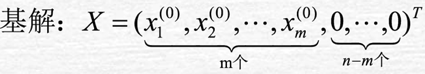
另非基变量 全部取值为0，则得到的一个解我们称之为基解。那么基解的个数最多为 （因为从A的n个列向量中任选线性无关的m个向量，所以每次组合得到的基向量B均对应着某一个基解）。同时满足 的解称之为基可行解。

基解，基可行解，可行解之间关系

令 ，则 ， 。此时目标函数值为 。

单纯形算法

介绍完上面的理论知识，下面介绍单纯形算法的基本思路。

基本思路为：从可行域的一个顶点到另一个顶点迭代求解。

基本可行解形式：

此处假设我们已经得到初始的一个基本可行解 （初始解求解后面会讲到）， 对应m个非零分量 ，且对应系数矩阵 中基向量为 ，这m个基向量之间是线性独立的，即 。

任选一个非基向量 ，则有 （因为矩阵A的秩为m，所以m+1个向量是线性相关的），令 ，此处 。这个参数 表示的是非零基变量 与 的最小比值（选择一个最小比值才能保证构造的新解 大于0）。第 个变量 称为出基变量，对应的A中基向量称为出基，第e个变量 称为入基变量（等会利用 构造新的解 的时候会把第 个变量变成非基变量，所以称为出基变量，相应的，第e个非基变量变成了基变量，称之为入基）。

构造新的解：

利用上述求得的参数 ，令 是基 对应的一组解，其中 ,即入基变量对应的系数为-1。下面证明 是上述线性规划问题的一个基本可行解。

因为 ，且 ，所以，即 是一个新的基本可行解。

举例说明如何构造新的解。

假设某一个线性规划的某一个基础可行解 和系数矩阵A如上图所示，此时基列向量为。如果选择非基列向量 （绿色）作为入基，则有 ，即 ,则 , ， 。所以通过选择非基向量 作为入基，构造了一个新的解（当然，此处还可以选择其他非基变量 ） 。新的基为 。那么问题来了，选择非基向量中的哪个向量作为入基比较好呢？通常我们希望目标函数越优越好。所以我们希望可以通过选择一个非基向量作为入基，使求得的目标函数变化最大。

选择入基向量：

前面假设我们已经有一个基本可行解 ， 并且系数矩阵A和约束系数c按照相同方式进行分块 （其实是x根据A进行分块）， 则对于线性规划问题

写成分块形式： ， ，因为 ，目标函数此时的值为 。

接下来考虑一个新的可行解 ， ，得到 ，新的可行解对应的目标函数值为

其中 ， ，表示对于着非基的位置。我们从中选择一个变量k ， 。令 ,并且同时有 ，则新的目标函数f’ < f ，这时候得到的新的基本可行解x’是优于之前的解x的。

但是我们希望每次尽可能的使目标函数 变得更优，所以我们每次选择 , 使得对应的 变化率最大。

上述的 称之为判别数或者检验数，所以如何选择入基向量的关键在于判断某一非基变量的对应的判别数是否大于0，然后从判别数大于0的非基变量中选择一个判别数最大的作为入基变量。这样其实就是一个转动(pivot)的过程

判断最优解：

当某一解x的所有非基变量对应的判别数均小于0时，该基本可行解为最优解。因为无法找到一个 ，使得目标函数值变得更加小。

求解初始基本可行解（两阶段法）

第一阶段：构造如下的线性规划问题

首先需要根据原线性规划问题的线性约束构造一个新的线性规划问题：

在原来约束的基础上加入变量 ,这样每个约束条件就变成了 。此处加入的 称之为人工变量。从而 ,可以写成 。很显然该线性规划问题对应着一个很明显的初始解 ，这就是构造该新方程组的原因。如果令 ，则 ，此时得到的x即为原线性规划问题的一个初始基本可行解。

所以新构造的线性规划问题的目标函数为 。在原线性规划问题有解 的前提下，只有当 时，该新的线性规划问题才有最优解。

证明：若存在 时目标函数有最优解，且此时有 ,存在 ，此时目标函数为 ，矛盾。

第二阶段：去掉人工变量，还原目标函数系数，用单纯形法求解即可
我们加入 的一个原因是该线性规划问题的一个明显的基本可行解是 ，即 （如果存在 ，利用所有行减去 最小的行，即可保证 ）。所以我们从初始解 ,使用单纯形法求得构造的线性规划问题的最优解。最优解可能的情形有如下几种：

1. ，此时原线性规划问题无解。
2. ，并且 的分量都是非基变量，这时的m个基变量都是原来的变量，此时的 就是原线性规划问题的一个最优解。
3. ，但 的某些分量是基变量，这时，可以用主元消元法，把原来变量 的分量引进基，替换出基变量中的人工变量。

收敛性

1. 当某一解x的所有非基变量对应的判别数均小于0时，该基本可行解为最优解。
2. 当最大判别数大于0对应的入基构造成的 都是小于0，此时任意取 都有 ，此时对应的解是无界的（unbound）.
3. 当最大判别数大于0且存在 ，此时可构造新的基本可行解。 ，所以此时 ，目标函数值下降。

综上分析，当极小化线性规划问题存在最优解时，对于非退化情形，在每次迭代中，均有 ，对应 ，经过迭代，目标函数值减少。由于基本可行解的个数有限，因此经过有限次迭代必能达到最优解。

表格形式单纯表法

我们将线性规划问题 ,变换成等价形式

从而有 ，用 左乘该式，与 相加，得到 ，从而原线性规划问题可以等价为如下形式:

将 的系数矩阵写成表格的形式

黑框表的上部分包含m个行，下半部分是一行。这样，经过单纯法之后的变换之后，表格的 即是入基变量 的值， 是目标函数值。

下面以一个具体的实例演示（两阶段法）。

首先引入松弛变量 ，将上述问题变成标准形式，再引入人工变量 ，得到一阶段问题。

初始解 ，非基向量对应检验数为 ，其中 , 。选择最大的检验数4，则 ，。令 ,选择 作为出基变量，对应的行为主行， 作为入基变量，对应的列为主列，此时第一行第二列对应的元素称为主元。我们需要把主列变成主元为1的单位向量。将第一行乘-2加到第二行，第一行乘0加到第三行，第一行乘-2加到第四行，然后第一行乘以1/2，这样就把第二列变成单位向量。得到新表如下：

此时虽然达到最优解（所有检验数小于0），但是人工变量 ,以零值出现在基变量中。需要在第二阶段开始之前把人工变量替换出去（人工变量变成非基变量总是对应最优解）。经过主元消去法得到下表

对应着原线性规划问题的一个解x = [0,1,0,0] .然后得到第二阶段初始表：

发现最大检验数为负值，此时解为最优解，且目标函数最优值为-1。

代码

Example qution: maximize —> 6x + 5y + 4z

      Subject to  2x + y + z <= 180    slack varibles  2x + y + z + s1 = 180  
          x + 3y + 2z <= 300                   x + 3y + 2z +s2 = 300
          2x + y + 2z <= 240                    2x + y + 2z +s3 = 240

you can make a arryas like below from this quetion:
colSizeA = 6 // input colmn size
rowSizeA = 3 // input row size
float C[N]={-6,-5,-4,0,0,0}; //Initialize the C array with the coefficients of the constraints of the objective function
float B[M]={180,300,240};//Initialize the B array constants of the constraints respectively

#include <iostream>
#include <cmath>
#include <vector>
using namespace std;

/*

The main method is in this program itself.

Instructions for compiling=>>

Run on any gcc compiler=>>

Special***** should compile in -std=c++11 or C++14 -std=gnu++11  *********  (mat be other versions syntacs can be different)

turorials point online compiler
==> go ti link   http://cpp.sh/ or  https://www.tutorialspoint.com/cplusplus/index.htm and click try it(scorel below) and after go to c++ editor copy code and paste.
after that click button execute.

if you have -std=c++11 you can run in command line;
g++ -o output Simplex.cpp
./output


How to give inputs to the program =>>>

   Example:
    colSizeA = 6 // input colmn size
    rowSizeA = 3  // input row size

    float C[N]={-6,-5,-4,0,0,0};  //Initialize the C array  with the coefficients of the constraints of the objective function
    float B[M]={240,360,300};//Initialize the B array constants of the constraints respectively


   //initialize the A array by giving all the coefficients of all the variables
   float A[M][N] =  {
                 { 2,  1,  1,   1,  0, 0},
                { 1,  3,  2,   0,  1, 0 },
                {   2,    1,  2,   0,  0,  1}
                };
*/


class Simplex{

    private:
    int rows, cols;
    //stores coefficients of all the variables
    std::vector <std::vector<float> > A;
    //stores constants of constraints
    std::vector<float> B;
    //stores the coefficients of the objective function
    std::vector<float> C;

    float maximum;

    bool isUnbounded;

    public:

    Simplex(std::vector <std::vector<float> > matrix,std::vector<float> b ,std::vector<float> c){
        maximum = 0;
        isUnbounded = false;
        rows = matrix.size();
        cols = matrix[0].size();
        A.resize( rows , vector<float>( cols , 0 ) );
        B.resize(b.size());
        C.resize(c.size());

        for(int i= 0;i<rows;i++){             //pass A[][] values to the metrix
            for(int j= 0; j< cols;j++ ){
                A[i][j] = matrix[i][j];

            }
        }

        for(int i=0; i< c.size() ;i++ ){      //pass c[] values to the B vector
            C[i] = c[i] ;
        }
        for(int i=0; i< b.size();i++ ){      //pass b[] values to the B vector
            B[i] = b[i];
        }

    }

    bool simplexAlgorithmCalculataion(){
        //check whether the table is optimal,if optimal no need to process further
        if(checkOptimality()==true){
            return true;
        }

        //find the column which has the pivot.The least coefficient of the objective function(C array).
        int pivotColumn = findPivotColumn();


        if(isUnbounded == true){
            cout<<"Error unbounded"<<endl;
            return true;
        }

        //find the row with the pivot value.The least value item's row in the B array
        int pivotRow = findPivotRow(pivotColumn);

        //form the next table according to the pivot value
        doPivotting(pivotRow,pivotColumn);

        return false;
    }

    bool checkOptimality(){
        //if the table has further negative constraints,then it is not optimal
        bool isOptimal = false;
        int positveValueCount = 0;

        //check if the coefficients of the objective function are negative
        for(int i=0; i<C.size();i++){
            float value = C[i];
            if(value >= 0){
                positveValueCount++;
            }
        }
        //if all the constraints are positive now,the table is optimal
        if(positveValueCount == C.size()){
            isOptimal = true;
            print();
        }
        return isOptimal;
    }

    void doPivotting(int pivotRow, int pivotColumn){

        float pivetValue = A[pivotRow][pivotColumn];//gets the pivot value

        float pivotRowVals[cols];//the column with the pivot

        float pivotColVals[rows];//the row with the pivot

        float rowNew[cols];//the row after processing the pivot value

        maximum = maximum - (C[pivotColumn]*(B[pivotRow]/pivetValue));  //set the maximum step by step
        //get the row that has the pivot value
        for(int i=0;i<cols;i++){
            pivotRowVals[i] = A[pivotRow][i];
        }
        //get the column that has the pivot value
        for(int j=0;j<rows;j++){
            pivotColVals[j] = A[j][pivotColumn];
        }

        //set the row values that has the pivot value divided by the pivot value and put into new row
        for(int k=0;k<cols;k++){
            rowNew[k] = pivotRowVals[k]/pivetValue;
        }

        B[pivotRow] = B[pivotRow]/pivetValue;


        //process the other coefficients in the A array by subtracting
        for(int m=0;m<rows;m++){
            //ignore the pivot row as we already calculated that
            if(m !=pivotRow){
                for(int p=0;p<cols;p++){
                    float multiplyValue = pivotColVals[m];
                    A[m][p] = A[m][p] - (multiplyValue*rowNew[p]);
                    //C[p] = C[p] - (multiplyValue*C[pivotRow]);
                    //B[i] = B[i] - (multiplyValue*B[pivotRow]);
                }

            }
        }

        //process the values of the B array
        for(int i=0;i<B.size();i++){
            if(i != pivotRow){

                float multiplyValue = pivotColVals[i];
                B[i] = B[i] - (multiplyValue*B[pivotRow]);

            }
        }
        //the least coefficient of the constraints of the objective function
        float multiplyValue = C[pivotColumn];
        //process the C array
        for(int i=0;i<C.size();i++){
            C[i] = C[i] - (multiplyValue*rowNew[i]);

        }

        //replacing the pivot row in the new calculated A array
        for(int i=0;i<cols;i++){
            A[pivotRow][i] = rowNew[i];
        }


    }

    //print the current A array
    void print(){
        for(int i=0; i<rows;i++){
            for(int j=0;j<cols;j++){
                cout<<A[i][j] <<" ";
            }
            cout<<""<<endl;
        }
        cout<<""<<endl;
    }

    //find the least coefficients of constraints in the objective function's position
    int findPivotColumn(){

        int location = 0;
        float minm = C[0];

        for(int i=1;i<C.size();i++){
            if(C[i]<minm){
                minm = C[i];
                location = i;
            }
        }

        return location;

    }

    //find the row with the pivot value.The least value item's row in the B array
    int findPivotRow(int pivotColumn){
        float positiveValues[rows];
        std::vector<float> result(rows,0);
        //float result[rows];
        int negativeValueCount = 0;

        for(int i=0;i<rows;i++){
            if(A[i][pivotColumn]>0){
                positiveValues[i] = A[i][pivotColumn];
            }
            else{
                positiveValues[i]=0;
                negativeValueCount+=1;
            }
        }
        //checking the unbound condition if all the values are negative ones
        if(negativeValueCount==rows){
            isUnbounded = true;
        }
        else{
            for(int i=0;i<rows;i++){
                float value = positiveValues[i];
                if(value>0){
                    result[i] = B[i]/value;

                }
                else{
                    result[i] = 0;
                }
            }
        }
        //find the minimum's location of the smallest item of the B array
        float minimum = 99999999;
        int location = 0;
        for(int i=0;i<sizeof(result)/sizeof(result[0]);i++){
            if(result[i]>0){
                if(result[i]<minimum){
                    minimum = result[i];

                    location = i;
                }
            }

        }

        return location;

    }

    void CalculateSimplex(){
        bool end = false;

        cout<<"initial array(Not optimal)"<<endl;
        print();

        cout<<" "<<endl;
        cout<<"final array(Optimal solution)"<<endl;

        while(!end){

            bool result = simplexAlgorithmCalculataion();

            if(result==true){

                end = true;


            }
        }
        cout<<"Answers for the Constraints of variables"<<endl;

        for(int i=0;i< A.size(); i++){  //every basic column has the values, get it form B array
            int count0 = 0;
            int index = 0;
            for(int j=0; j< rows; j++){
                if(A[j][i]==0.0){
                    count0 += 1;
                }
                else if(A[j][i]==1){
                    index = j;
                }

            }

            if(count0 == rows -1 ){

                cout<<"variable"<<index+1<<": "<<B[index]<<endl;  //every basic column has the values, get it form B array
            }
            else{
                cout<<"variable"<<index+1<<": "<<0<<endl;

            }

        }

        cout<<""<<endl;
        cout<<"maximum value: "<<maximum<<endl;  //print the maximum values

    }

};

int main()
{

    int colSizeA=6;  //should initialise columns size in A
    int rowSizeA = 3;  //should initialise columns row in A[][] vector

    float C[]= {-6,-5,-4,0,0,0};  //should initialis the c arry here
    float B[]={180,300,240};  // should initialis the b array here

    float a[3][6] = {    //should intialis the A[][] array here
        { 2,  1,  1, 1, 0, 0},
        { 1,  3,  2, 0, 1, 0},
        { 2,  1,  2, 0, 0, 1}
    };

    std::vector <std::vector<float> > vec2D(rowSizeA, std::vector<float>(colSizeA, 0));

    std::vector<float> b(rowSizeA,0);
    std::vector<float> c(colSizeA,0);

    for(int i=0;i<rowSizeA;i++){         //make a vector from given array
        for(int j=0; j<colSizeA;j++){
            vec2D[i][j] = a[i][j];
        }
    }

    for(int i=0;i<rowSizeA;i++){
        b[i] = B[i];
    }

    for(int i=0;i<colSizeA;i++){
        c[i] = C[i];
    }


    // hear the make the class parameters with A[m][n] vector b[] vector and c[] vector
    Simplex simplex(vec2D,b,c);
    simplex.CalculateSimplex();

    return 0;
}

参考文献《最优化理论与算法》