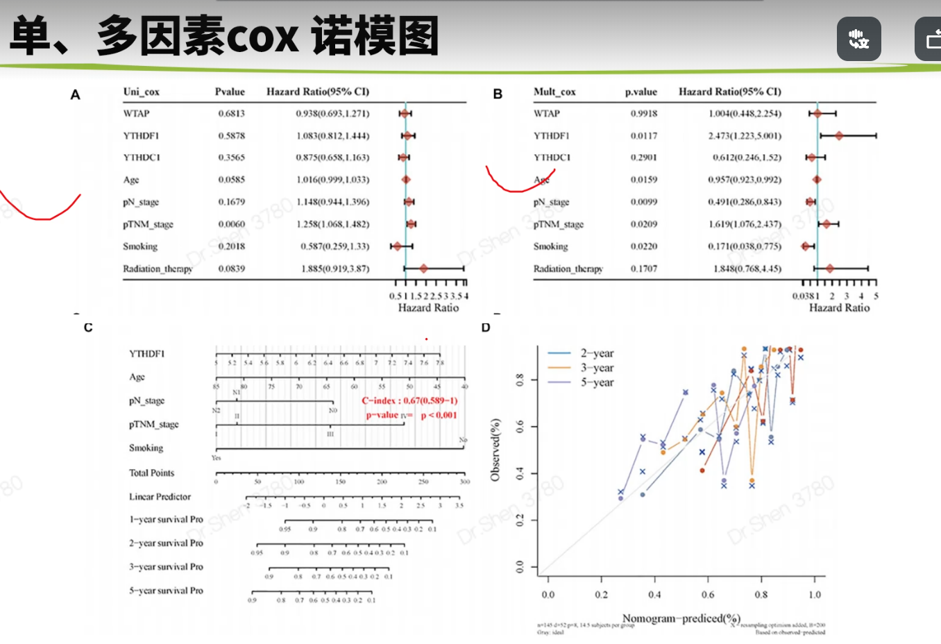
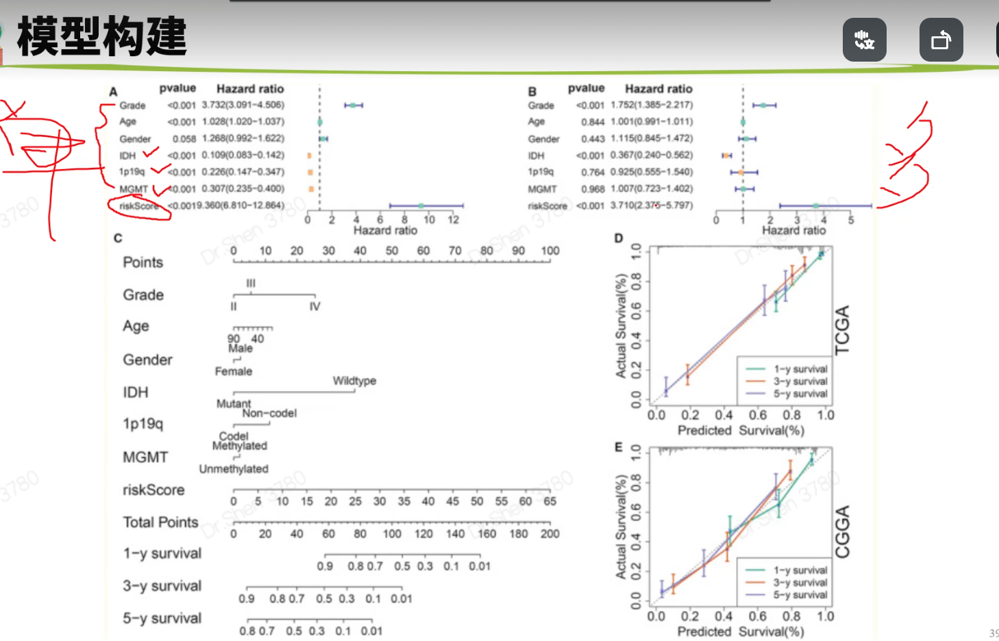
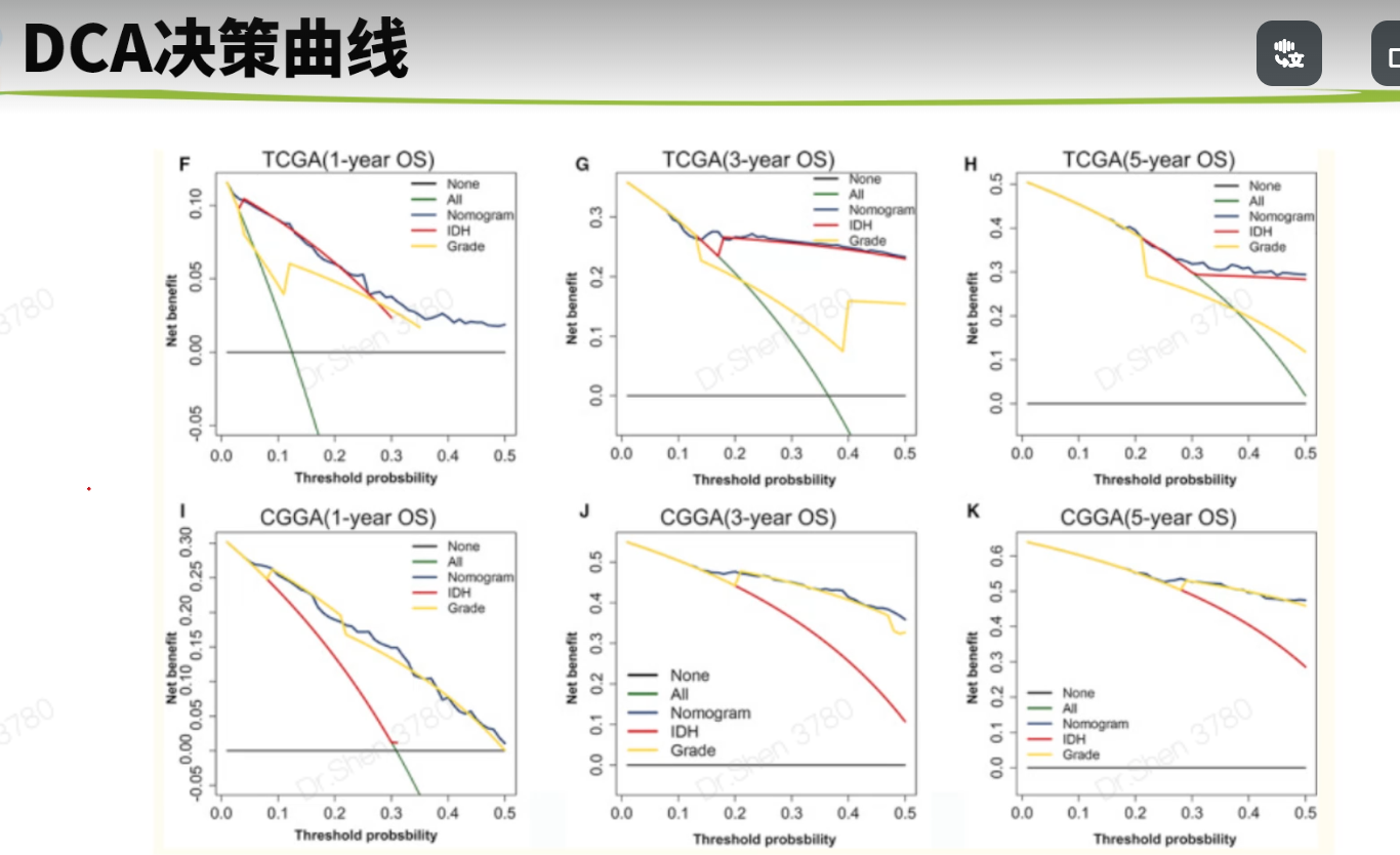
模型可视化生信技能树1.简版森林图#https://zhuanlan.zhihu.com/p/109401314rm(list = ls())load("../1_data_pre/exp_surv1.Rdata")rm(surv1)load("../3_anno_immu/TCGA_idh.Rdata")library(stringr)surv1 = idh[,c("event","time","fp","IDH","age","gender","grade","Meth","1p19q")]colnames(surv1)[3] = "riskScore"library(survival)library(survminer)model1 = coxph(Surv(time,event)~.,data = surv1)ggforest(model1,data = surv1)coxdat = surv1table(coxdat$IDH)#### Mutant WT## 435 246coxdat$IDH = ifelse(coxdat$IDH=="WT",1,2)table(coxdat$gender)#### female male## 267 364coxdat$gender = ifelse(coxdat$gender=="female",1,2)table(coxdat$grade)#### G2 G3 G4## 222 242 167coxdat$grade = ifelse(coxdat$grade=="G2",2,ifelse(coxdat$grade=="G3",3,4))table(coxdat$Meth)#### Methylated Unmethylated## 488 165coxdat$Meth = ifelse(coxdat$Meth=="Unmethylated",1,2)str(coxdat)## 'data.frame': 691 obs. of 9 variables:## $ event : int 1 1 0 0 0 1 1 1 1 1 ...## $ time : int 441 74 459 463 485 1427 1427 1009 388 759 ...## $ riskScore: num 10.9 11.3 10.1 11 11.7 ...## $ IDH : num 1 1 2 1 1 1 1 2 1 1 ...## $ age : num 78 62 43 53 64 63 63 30 54 49 ...## $ gender : num 2 1 2 2 2 1 1 2 2 2 ...## $ grade : num 4 4 4 4 4 4 4 4 4 4 ...## $ Meth : num 1 1 2 1 1 2 2 2 1 NA ...## $ 1p19q : chr "non-codel" "non-codel" "non-codel" "non-codel" ...coxdat$`1p19q` = ifelse(coxdat$`1p19q`=="non-codel",1,2)model = coxph(Surv(time,event)~.,data = coxdat)ggforest(model,data = coxdat)2.美化版森林图单因素coxlibrary(tinyarray)dat1 = surv_cox(t(coxdat[,3:8]),coxdat,continuous = T,pvalue_cutoff = 1)dat2 = as.data.frame(dat1[,c("HR","HRCILL","HRCIUL","p")])datp = format(round(dat2[,1:3],3),nsmall = 3)dat2$Trait = rownames(dat1)dat2$HR2 = paste0(datp[, 1], "(", datp[, 2], "-", datp[, 3], ")")str(dat2)## 'data.frame': 6 obs. of 6 variables:## $ HR : num 2.688 0.115 1.072 1.101 4.776 ...## $ HRCILL: num 2.3899 0.0835 1.0602 0.8323 3.7853 ...## $ HRCIUL: num 3.023 0.158 1.084 1.456 6.025 ...## $ p : num 0 0 0 0.501 0 ...## $ Trait : chr "riskScore" "IDH" "age" "gender" ...## $ HR2 : chr "2.688(2.390-3.023)" "0.115(0.083-0.158)" "1.072(1.060-1.084)" "1.101(0.832-1.456)" ...dat2$p = ifelse(dat2$p<0.001,"<0.001",format(round(dat2$p,3),nsmall = 3))library(forestplot)forestplot(dat2[, c(5, 4, 6)],mean = dat2[, 1],lower = dat2[, 2],upper = dat2[, 3],zero = 1,boxsize = 0.2,col = fpColors(box = '#1075BB', lines = 'black', zero = 'grey'),lty.ci = "solid",graph.pos = 4)多因素coxm = summary(model)p = ifelse(m$coefficients[, 5] <= 0.001,"<0.001",ifelse(m$coefficients[, 5] <= 0.01,"<0.01",ifelse(m$coefficients[, 5] <= 0.05,paste(round(m$coefficients[, 5], 3), " *"),round(m$coefficients[, 5], 3))))#HR和它的置信区间dat2 = as.data.frame(round(m$conf.int[, c(1, 3, 4)], 2))dat2 = tibble::rownames_to_column(dat2, var = "Trait")colnames(dat2)[2:4] = c("HR", "lower", "upper")#需要在图上显示的HR文字和p值dat2$HR2 = paste0(dat2[, 2], "(", dat2[, 3], "-", dat2[, 4], ")")dat2$p = pstr(dat2)## 'data.frame': 7 obs. of 6 variables:## $ Trait: chr "riskScore" "IDH" "age" "gender" ...## $ HR : num 2.43 1.22 1.05 1.29 0.97 0.72 0.68## $ lower: num 1.96 0.68 1.03 0.93 0.69 0.5 0.37## $ upper: num 3.02 2.19 1.06 1.8 1.35 1.05 1.24## $ HR2 : chr "2.43(1.96-3.02)" "1.22(0.68-2.19)" "1.05(1.03-1.06)" "1.29(0.93-1.8)" ...## $ p : chr "<0.001" "0.507" "<0.001" "0.129" ...forestplot(dat2[, c(1, 5, 6)],mean = dat2[, 2],lower = dat2[, 3],upper = dat2[, 4],zero = 1,boxsize = 0.4,col = fpColors(box = '#1075BB', lines = 'black', zero = 'grey'),lty.ci = "solid",graph.pos = 4)3.诺模图library(rms)dd<-datadist(surv1)options(datadist="dd")mod <- cph(as.formula(paste("Surv(time, event) ~ ",paste(colnames(surv1)[3:8],collapse = "+"))),data=surv1,x=T,y=T,surv = T)surv<-Survival(mod)m1<-function(x) surv(365,x)m3<-function(x) surv(1095,x)m5<-function(x) surv(1825,x)x<-nomogram(mod,fun = list(m1,m3,m5),funlabel = c('1-y survival','3-y survival','5-y survival'),lp = F)plot(x)奇怪的结果sfit1 = survival::survfit(survival::Surv(time, event) ~grade, data = surv1)survminer::ggsurvplot(sfit1, pval = TRUE, palette = "jco", data = surv1, legend = c(0.8, 0.8))对此的进一步探索:https://www.yuque.com/xiaojiewanglezenmofenshen/bsgk2d/ci7604f1 <- cph(formula = as.formula(paste("Surv(time, event) ~ ",paste(colnames(surv1)[3:8],collapse = "+"))),data=surv1,x=T,y=T,surv = T, time.inc=365)cal1 <- calibrate(f1, cmethod="KM", method="boot", u=365, m=50, B=1000)## Using Cox survival estimates at 365 Daysf3 <- cph(formula = as.formula(paste("Surv(time, event) ~ ",paste(colnames(surv1)[3:8],collapse = "+"))),data=surv1,x=T,y=T,surv = T, time.inc=1095)cal3 <- calibrate(f3, cmethod="KM", method="boot", u=1095, m=50, B=1000)## Using Cox survival estimates at 1095 Daysf5 <- cph(formula = as.formula(paste("Surv(time, event) ~ ",paste(colnames(surv1)[3:8],collapse = "+"))),data=surv1,x=T,y=T,surv = T, time.inc=1825)cal5 <- calibrate(f5, cmethod="KM", method="boot", u=1825, m=50, B=1000)## Using Cox survival estimates at 1825 Daysplot(cal1,lwd = 2,lty = 0,errbar.col = c("#92C5DE"),bty = "l", #只画左边和下边框xlim = c(0,1),ylim= c(0,1),xlab = "Nomogram-prediced OS (%)",ylab = "Observed OS (%)",col = c("#92C5DE"),cex.lab=1.2,cex.axis=1, cex.main=1.2, cex.sub=0.6)lines(cal3[,c('mean.predicted',"KM")],type = 'b', lwd = 2, col = c("#92C5DE"), pch = 16)mtext("")plot(cal3,lwd = 2,lty = 0,errbar.col = c("#F4A582"),bty = "l", #只画左边和下边框xlim = c(0,1),ylim= c(0,1),xlab = "Nomogram-prediced OS (%)",ylab = "Observed OS (%)",col = c("#F4A582"),cex.lab=1.2,cex.axis=1, cex.main=1.2, cex.sub=0.6)lines(cal3[,c('mean.predicted',"KM")],type = 'b', lwd = 2, col = c("#F4A582"), pch = 16)mtext("")plot(cal5,lwd = 2,lty = 0,errbar.col = c("#66C2A5"),xlim = c(0,1),ylim= c(0,1),col = c("#66C2A5"),add = T)lines(cal5[,c('mean.predicted',"KM")],type = 'b', lwd = 2, col = c("#66C2A5"), pch = 16)abline(0,1, lwd = 2, lty = 3, col = c("#224444"))legend("bottomright", #图例的位置legend = c("1-y survival","3-y survival","5-y survival"), #图例文字col = c("#92C5DE", "#F4A582", "#66C2A5"), #图例线的颜色,与文字对应lwd = 2,#图例中线的粗细cex = 1.2)4.DCA曲线#devtools::install_github('yikeshu0611/ggDCA')dat = surv1dat$nomo = predict(model1,newdata = dat)library(ggDCA)library(rms)nomo <- cph(Surv(time,event)~nomo,dat)IDH <- cph(Surv(time,event)~IDH,dat)Grade <- cph(Surv(time,event)~grade,dat)data <- dca(nomo,IDH,Grade)ggplot(data)
文献1 肺癌
该文献问题比较多,注意入坑
配对样本的数据,注意配色、图标
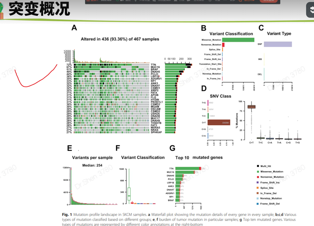
突变分析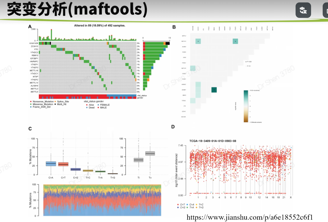
文献2 黑色素瘤
寻找上述资料
xuna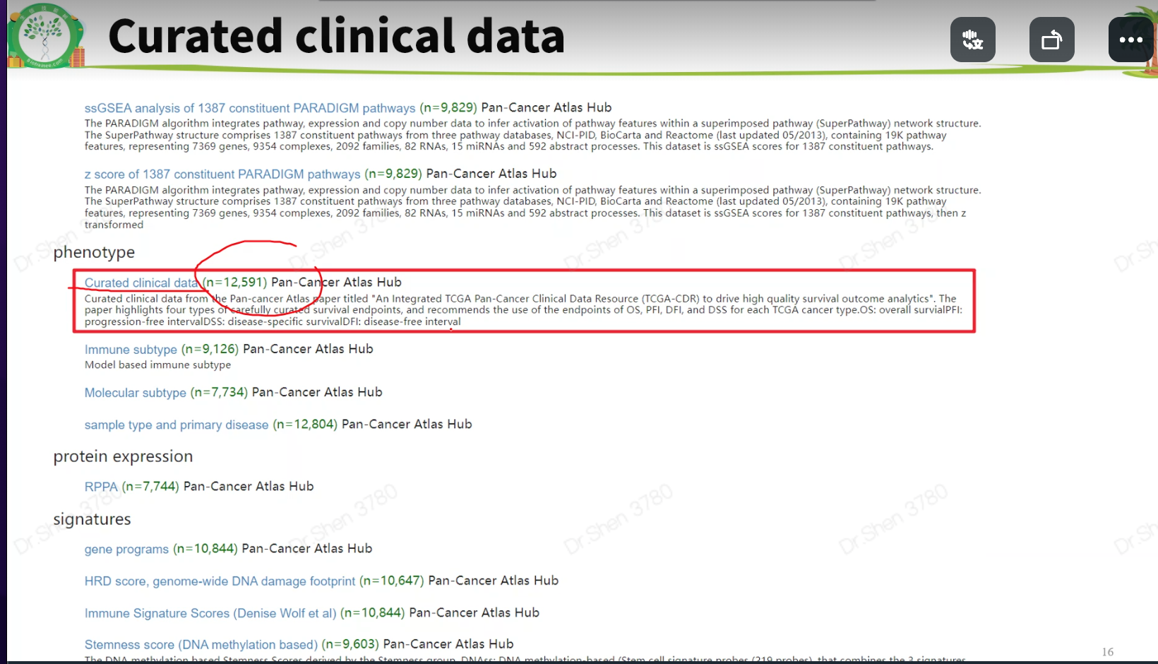
其他方法计算肿瘤纯度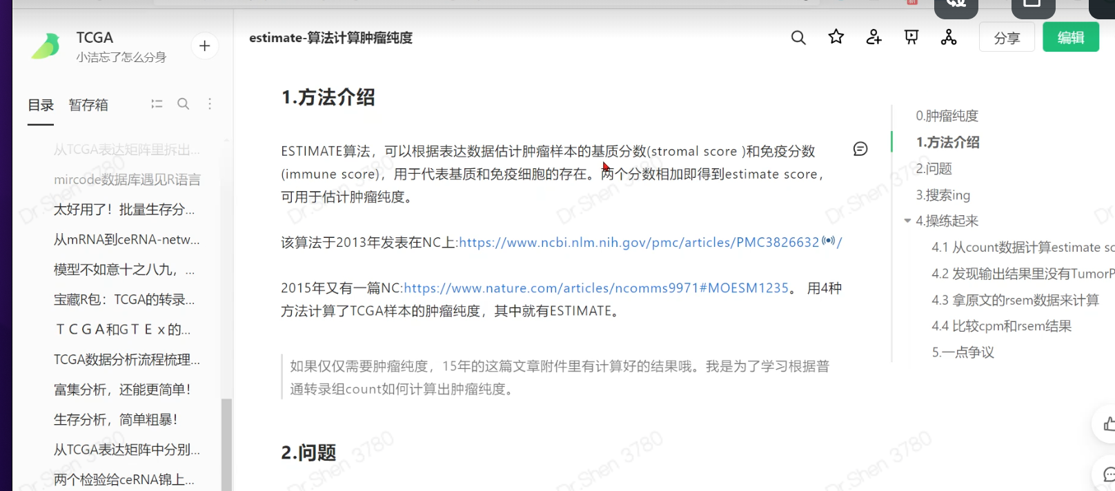
免疫浸润:Timer 或 cibersort 或 ssgsea
文献3 胶质瘤
图好看,但逻辑有些问题
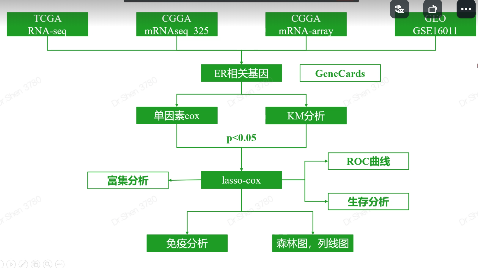
step1_数据收集1.数据整理的说明1.1 下载的数据四个数据的表达矩阵、生存信息表格。TCGA的LGG和GBM是分开的。后续用代码合并到一起。1.2 表达矩阵的要求(1)就要是取过log、没有异常值的矩阵,标准化过的也可以,因为不做差异分析。(2)如果是转录组数据,要log之后的标准化数据。(因为这里只做生存分析,不做差异分析,所以没有必要找count数据)(3)行名都转换成gene symbol(4)只要tumor样本,不要normal1.3 临床信息的要求(1)要有每个样本对应的生存时间和结局事件,并用代码调整顺序,与表达矩阵的样本顺序相同,严格一一对应。(2)为了后续代码统一,把生存时间和结局事件列名统一起来,都叫“time”和“event”。(3)至于时间的单位,反正是分别计算的,统不统一无所谓。1.4 关于数据来源的说明数据来源于哪个数据库,不是主要矛盾。重点是分清楚是芯片数据还是转录组数据,是芯片的话要能找到探针注释。如果是转录组数据,则需要分清楚是否标准化,进行了哪种标准化。反正是分别分析,又不需要合并,所以直接使用即可。2.TCGA的RNA-seq数据Table S1显示样本数量691,TCGA的GBM数据173样本,LGG有529样本。2.1 TCGA表达矩阵exp_gbm = read.table("TCGA-GBM.htseq_fpkm.tsv.gz",header = T,row.names = 1,check.names = F)exp_lgg = read.table("TCGA-LGG.htseq_fpkm.tsv.gz",header = T,row.names = 1,check.names = F)exp1 = as.matrix(cbind(exp_gbm,exp_lgg))#行名转换为gene symbollibrary(stringr)library(AnnoProbe)rownames(exp1) = str_split(rownames(exp1),"\\.",simplify = T)[,1];head(rownames(exp1))## [1] "ENSG00000242268" "ENSG00000270112" "ENSG00000167578" "ENSG00000273842"## [5] "ENSG00000078237" "ENSG00000146083"re = annoGene(rownames(exp1),ID_type = "ENSEMBL");head(re)## SYMBOL biotypes ENSEMBL chr start## 1 DDX11L1 transcribed_unprocessed_pseudogene ENSG00000223972 chr1 11869## 2 WASH7P unprocessed_pseudogene ENSG00000227232 chr1 14404## 3 MIR6859-1 miRNA ENSG00000278267 chr1 17369## 4 MIR1302-2HG lncRNA ENSG00000243485 chr1 29554## 6 FAM138A lncRNA ENSG00000237613 chr1 34554## 7 OR4G4P unprocessed_pseudogene ENSG00000268020 chr1 52473## end## 1 14409## 2 29570## 3 17436## 4 31109## 6 36081## 7 53312library(tinyarray)exp1 = trans_array(exp1,ids = re,from = "ENSEMBL",to = "SYMBOL")exp1[1:4,1:4]## TCGA-06-0878-01A TCGA-26-5135-01A TCGA-06-5859-01A TCGA-06-2563-01A## DDX11L1 0.0000000 0.0221755 0.00000000 0.01797799## WASH7P 0.6673943 1.7429940 0.65334641 1.57566444## MIR6859-1 1.2006708 2.1880585 1.51229174 2.17610561## MIR1302-2HG 0.0000000 0.0000000 0.02520857 0.00000000dim(exp1)## [1] 56514 702#删除正常样本Group = make_tcga_group(exp1)table(Group)## Group## normal tumor## 5 697exp1 = exp1[,Group == "tumor"]#过滤表达量0值太多的基因exp1 = exp1[apply(exp1, 1, function(x){sum(x>0)>200}),]2.2 TCGA生存信息surv_gbm = readr::read_tsv("TCGA-GBM.survival.tsv")surv_gbm$TYPE = "GBM"surv_lgg = readr::read_tsv("TCGA-LGG.survival.tsv")surv_lgg$TYPE = "LGG"surv1 = rbind(surv_gbm,surv_lgg)head(surv1)## # A tibble: 6 x 5## sample OS `_PATIENT` OS.time TYPE## <chr> <dbl> <chr> <dbl> <chr>## 1 TCGA-12-0657-01A 1 TCGA-12-0657 3 GBM## 2 TCGA-32-1977-01A 0 TCGA-32-1977 3 GBM## 3 TCGA-19-1791-01A 0 TCGA-19-1791 4 GBM## 4 TCGA-28-1757-01A 0 TCGA-28-1757 4 GBM## 5 TCGA-19-2624-01A 1 TCGA-19-2624 5 GBM## 6 TCGA-41-4097-01A 1 TCGA-41-4097 6 GBMtable(colnames(exp1) %in% surv1$sample)#### FALSE TRUE## 6 691s = intersect(colnames(exp1),surv1$sample)exp1 = exp1[,s]surv1 = surv1[match(s,surv1$sample),]colnames(surv1)[c(2,4)] = c("event","time")exp1[1:4,1:4]## TCGA-06-0878-01A TCGA-26-5135-01A TCGA-06-5859-01A TCGA-06-2563-01A## WASH7P 0.66739425 1.74299400 0.65334641 1.57566444## MIR6859-1 1.20067078 2.18805848 1.51229174 2.17610561## AL627309.1 0.00000000 0.02066275 0.01386984 0.00000000## CICP27 0.09691981 0.01013527 0.00000000 0.02449211head(surv1)## # A tibble: 6 x 5## sample event `_PATIENT` time TYPE## <chr> <dbl> <chr> <dbl> <chr>## 1 TCGA-06-0878-01A 0 TCGA-06-0878 218 GBM## 2 TCGA-26-5135-01A 1 TCGA-26-5135 270 GBM## 3 TCGA-06-5859-01A 0 TCGA-06-5859 139 GBM## 4 TCGA-06-2563-01A 0 TCGA-06-2563 932 GBM## 5 TCGA-41-2571-01A 1 TCGA-41-2571 26 GBM## 6 TCGA-28-5207-01A 1 TCGA-28-5207 343 GBMidentical(colnames(exp1),surv1$sample)## [1] TRUE共691个有生存信息的tumor样本。3.CGGA芯片数据整理exp2 = read.table("CGGA/CGGA.mRNA_array_301_gene_level.20200506.txt",header = T,row.names = 1)surv2 = read.table("CGGA/CGGA.mRNA_array_301_clinical.20200506.txt",sep = "\t",header = T,check.names = F)head(surv2)## CGGA_ID TCGA_subtypes PRS_type Histology Grade Gender Age OS## 1 CGGA_11 Classical Primary GBM WHO IV Female 57 155## 2 CGGA_124 Mesenchymal Primary GBM WHO IV Male 53 414## 3 CGGA_126 Mesenchymal Primary GBM WHO IV Female 50 1177## 4 CGGA_168 Mesenchymal Primary GBM WHO IV Male 17 3086## 5 CGGA_172 Mesenchymal Primary GBM WHO IV Female 57 462## 6 CGGA_195 Mesenchymal Primary GBM WHO IV Male 48 486## Censor (alive=0; dead=1) Radio_status (treated=1;un-treated=0)## 1 1 1## 2 1 1## 3 1 1## 4 0 1## 5 1 1## 6 1 1## Chemo_status (TMZ treated=1;un-treated=0) IDH_mutation_status## 1 0 Wildtype## 2 0 Wildtype## 3 1 Wildtype## 4 1 Wildtype## 5 0 Wildtype## 6 1 Wildtype## 1p19q_Codeletion_status MGMTp_methylation_status## 1 <NA> un-methylated## 2 <NA> un-methylated## 3 <NA> un-methylated## 4 <NA> un-methylated## 5 <NA> un-methylated## 6 <NA> un-methylateds = intersect(surv2$CGGA_ID,colnames(exp2))exp2 = as.matrix(exp2[,s])surv2 = surv2[match(s,surv2$CGGA_ID),]colnames(surv2)[c(9,8)] = c("event","time")exp2[1:4,1:4]## CGGA_11 CGGA_124 CGGA_126 CGGA_168## A1BG -0.3603635 0.5649519 0.3047719 0.1749144## A1CF 2.3413600 1.1707935 2.2081513 0.9652286## A2BP1 0.0345194 1.0964074 0.3024883 0.0949111## A2LD1 -0.9130564 0.5108800 0.4253669 -0.1949377head(surv2)## CGGA_ID TCGA_subtypes PRS_type Histology Grade Gender Age time event## 1 CGGA_11 Classical Primary GBM WHO IV Female 57 155 1## 2 CGGA_124 Mesenchymal Primary GBM WHO IV Male 53 414 1## 3 CGGA_126 Mesenchymal Primary GBM WHO IV Female 50 1177 1## 4 CGGA_168 Mesenchymal Primary GBM WHO IV Male 17 3086 0## 5 CGGA_172 Mesenchymal Primary GBM WHO IV Female 57 462 1## 6 CGGA_195 Mesenchymal Primary GBM WHO IV Male 48 486 1## Radio_status (treated=1;un-treated=0)## 1 1## 2 1## 3 1## 4 1## 5 1## 6 1## Chemo_status (TMZ treated=1;un-treated=0) IDH_mutation_status## 1 0 Wildtype## 2 0 Wildtype## 3 1 Wildtype## 4 1 Wildtype## 5 0 Wildtype## 6 1 Wildtype## 1p19q_Codeletion_status MGMTp_methylation_status## 1 <NA> un-methylated## 2 <NA> un-methylated## 3 <NA> un-methylated## 4 <NA> un-methylated## 5 <NA> un-methylated## 6 <NA> un-methylatedidentical(surv2$CGGA_ID,colnames(exp2))## [1] TRUE4.CGGA转录组数据整理exp3 = read.table("CGGA/CGGA.mRNAseq_325.RSEM-genes.20200506.txt",header = T,row.names = 1)exp3 = as.matrix(log2(exp3+1))surv3 = read.table("CGGA/CGGA.mRNAseq_325_clinical.20200506.txt",sep = "\t",header = T,check.names = F)head(surv3)## CGGA_ID PRS_type Histology Grade Gender Age OS## 1 CGGA_1001 Primary GBM WHO IV Male 11 3817## 2 CGGA_1006 Primary AA WHO III Male 42 254## 3 CGGA_1007 Primary GBM WHO IV Female 57 345## 4 CGGA_1011 Primary GBM WHO IV Female 46 109## 5 CGGA_1015 Primary GBM WHO IV Male 62 164## 6 CGGA_1019 Recurrent rGBM WHO IV Male 60 212## Censor (alive=0; dead=1) Radio_status (treated=1;un-treated=0)## 1 0 0## 2 1 1## 3 1 1## 4 1 1## 5 1 1## 6 1 0## Chemo_status (TMZ treated=1;un-treated=0) IDH_mutation_status## 1 1 Wildtype## 2 1 Wildtype## 3 1 Wildtype## 4 0 Wildtype## 5 0 Wildtype## 6 1 Wildtype## 1p19q_codeletion_status MGMTp_methylation_status## 1 Non-codel un-methylated## 2 Non-codel un-methylated## 3 Non-codel un-methylated## 4 Non-codel un-methylated## 5 Non-codel un-methylated## 6 Non-codel methylatedcolnames(surv3)[c(8,7)] = c("event","time")s = intersect(surv3$CGGA_ID,colnames(exp3))exp3 = exp3[,s]surv3 = surv3[match(s,surv3$CGGA_ID),]exp3[1:4,1:4]## CGGA_1001 CGGA_1006 CGGA_1007 CGGA_1011## A1BG 3.769772 3.0054000 4.958379 2.933573## A1BG-AS1 1.641546 1.0908534 2.933573 2.411426## A2M 8.826294 6.7487296 7.698357 9.467952## A2M-AS1 2.104337 0.1763228 0.704872 1.384050head(surv3)## CGGA_ID PRS_type Histology Grade Gender Age time event## 1 CGGA_1001 Primary GBM WHO IV Male 11 3817 0## 2 CGGA_1006 Primary AA WHO III Male 42 254 1## 3 CGGA_1007 Primary GBM WHO IV Female 57 345 1## 4 CGGA_1011 Primary GBM WHO IV Female 46 109 1## 5 CGGA_1015 Primary GBM WHO IV Male 62 164 1## 6 CGGA_1019 Recurrent rGBM WHO IV Male 60 212 1## Radio_status (treated=1;un-treated=0)## 1 0## 2 1## 3 1## 4 1## 5 1## 6 0## Chemo_status (TMZ treated=1;un-treated=0) IDH_mutation_status## 1 1 Wildtype## 2 1 Wildtype## 3 1 Wildtype## 4 0 Wildtype## 5 0 Wildtype## 6 1 Wildtype## 1p19q_codeletion_status MGMTp_methylation_status## 1 Non-codel un-methylated## 2 Non-codel un-methylated## 3 Non-codel un-methylated## 4 Non-codel un-methylated## 5 Non-codel un-methylated## 6 Non-codel methylatedidentical(surv3$CGGA_ID,colnames(exp3))## [1] TRUE我没仔细看这个表达矩阵具体是哪种标准化,反正这个数据只是作为例子,我们就不深究到底是啥了,直接拿来用。注意如果是自己要用来发文章的数据,是要看清楚的,没标准化需要自行标准化,cpm,tmp,fpkm都行。5.GSE16011的整理library(tinyarray)geo = geo_download("GSE16011")library(stringr)#只要tumor样本k = str_detect(geo$pd$title,"glioma");table(k)## k## FALSE TRUE## 8 276geo$exp = geo$exp[,k]geo$pd = geo$pd[k,]# 把行名转换为gene symbolgpl = GEOquery::getGEO(filename = "GPL8542_family.soft.gz",destdir = ".")ids = gpl@dataTable@table[,1:2]library(clusterProfiler)library(org.Hs.eg.db)e2s = bitr(ids$ORF,fromType = "ENTREZID",toType = "SYMBOL",OrgDb = "org.Hs.eg.db")ids = merge(ids,e2s,by.x = "ORF",by.y = "ENTREZID")ids = ids[,2:3]colnames(ids) = c("probe_id","symbol")exp4 = trans_array(geo$exp,ids)surv4 = geo$pd[,c(1,4,7,9)]exp4[1:4,1:4]## GSM405201 GSM405202 GSM405203 GSM405204## A1BG 7.219401 6.031261 6.707681 6.330666## A2M 12.206626 13.260587 12.352693 13.044375## NAT1 5.182989 7.213272 6.570733 6.343490## NAT2 5.239842 5.260373 5.697435 4.859682head(surv4)## title age at diagnosis:ch1 histology:ch1 gender:ch1## GSM405201 glioma 8 44.57 OD (grade III) Female## GSM405202 glioma 9 28.69 OD (grade III) Male## GSM405203 glioma 11 38.58 OD (grade III) Male## GSM405204 glioma 13 33.89 OD (grade III) Male## GSM405205 glioma 20 48.03 OD (grade III) Male## GSM405206 glioma 21 31.53 OD (grade III) Maleidentical(rownames(surv4),colnames(exp4))## [1] TRUE临床信息表格里没有生存信息,所以从文章附件里找从文章附件里提取临床信息表格https://aacrjournals.org/cancerres/article/69/23/9065/553005/Intrinsic-Gene-Expression-Profiles-of-Gliomas-Are包非常难装,需要配置java,但这个需求不常用,直接跳过这个过程。if(!file.exists("exp_surv4.Rdata")){library(tabulizer)f <- "00085472can092307-sup-stabs_1-6.pdf"re <- extract_tables(f,pages = 1:10) #提取前10页的表格。str(re)re = do.call(rbind,re)re[1:4,1:4]colnames(re) = re[1,]re = re[-1,]re = data.frame(re)re[re==""]=NAlibrary(readr)re$Survival..years. = parse_double(re$Survival..years.,locale = locale(decimal_mark = ","))re$Age.at.diagnosis = parse_double(re$Age.at.diagnosis,locale = locale(decimal_mark = ","))dim(exp4)k = re$Reviewed.histological.diagnosis!="control";table(k)re = re[k,]re$Database.number = paste("glioma",re$Database.number)surv4$ID = rownames(surv4)surv4 = merge(surv4,re,by.x = "title",by.y = "Database.number")colnames(surv4)[13:14] = c("event","time")table(surv4$event)surv4$time = as.integer(surv4$time*365) #天为单位surv4$event[surv4$event=="Lost to\rfollow up"]=NAtable(surv4$event)surv4$event=ifelse(surv4$event=="Alive",0,1)head(surv4)s = intersect(surv4$ID,colnames(exp4))exp4 = exp4[,s]surv4 = surv4[match(s,surv4$ID),]save(exp4,surv4,file = "exp_surv4.Rdata")}load("exp_surv4.Rdata")exp4[1:4,1:4]## GSM405234 GSM405235 GSM405236 GSM405237## A1BG 7.613150 6.995666 7.337393 6.287498## A2M 13.166457 13.003225 13.814942 12.991301## NAT1 5.581672 7.470894 7.845210 6.088651## NAT2 5.206464 4.618245 4.881652 5.011908head(surv4)## title age at diagnosis:ch1 histology:ch1 gender:ch1 ID Gender## 1 glioma 101 57.68 GBM (grade IV) Female GSM405234 Female## 2 glioma 104 71.09 GBM (grade IV) Male GSM405235 Male## 3 glioma 105 52.20 GBM (grade IV) Male GSM405236 Male## 4 glioma 107 51.17 GBM (grade IV) Male GSM405237 Male## 5 glioma 11 38.58 OD (grade III) Male GSM405203 Male## 6 glioma 111 37.25 GBM (grade IV) Male GSM405238 Male## Reviewed.histological.diagnosis Age.at.diagnosis KPS Type.of.surgery## 1 GBM (grade IV) 57.68 70 Partial resection## 2 GBM (grade IV) 71.09 80 Partial resection## 3 GBM (grade IV) 52.20 80 Complete resection## 4 GBM (grade IV) 51.17 70 Stereotactic biopsy## 5 OD (grade III) 38.58 <NA> Complete resection## 6 GBM (grade IV) 37.25 80 Stereotactic biopsy## Radiotherapy Chemotherapy event time## 1 yes no 1 226## 2 yes no 1 76## 3 yes no 1 375## 4 yes no 1 149## 5 yes no 1 3255## 6 yes no 1 343identical(surv4$ID,colnames(exp4))## [1] TRUE检查和保存数据par(mfrow = c(2,2))boxplot(exp1[,1:10])boxplot(exp2[,1:10])boxplot(exp3[,1:10])boxplot(exp4[,1:10])save(exp1,surv1,file = "exp_surv1.Rdata")save(exp2,surv2,file = "exp_surv2.Rdata")save(exp3,surv3,file = "exp_surv3.Rdata")save(exp4,surv4,file = "exp_surv4.Rdata")
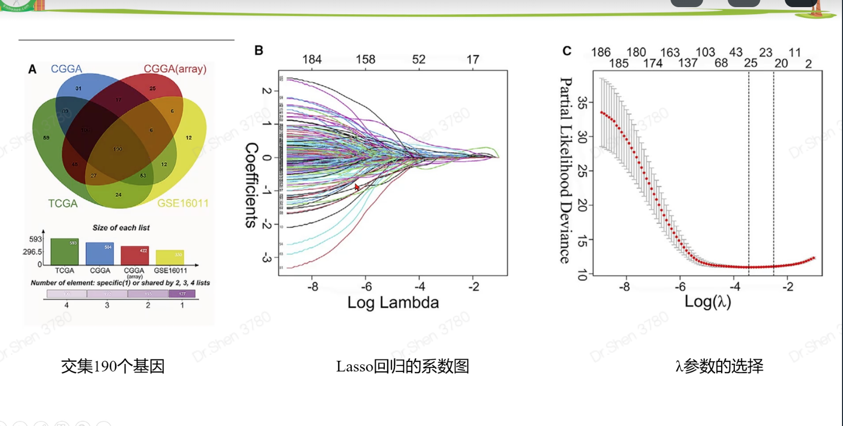
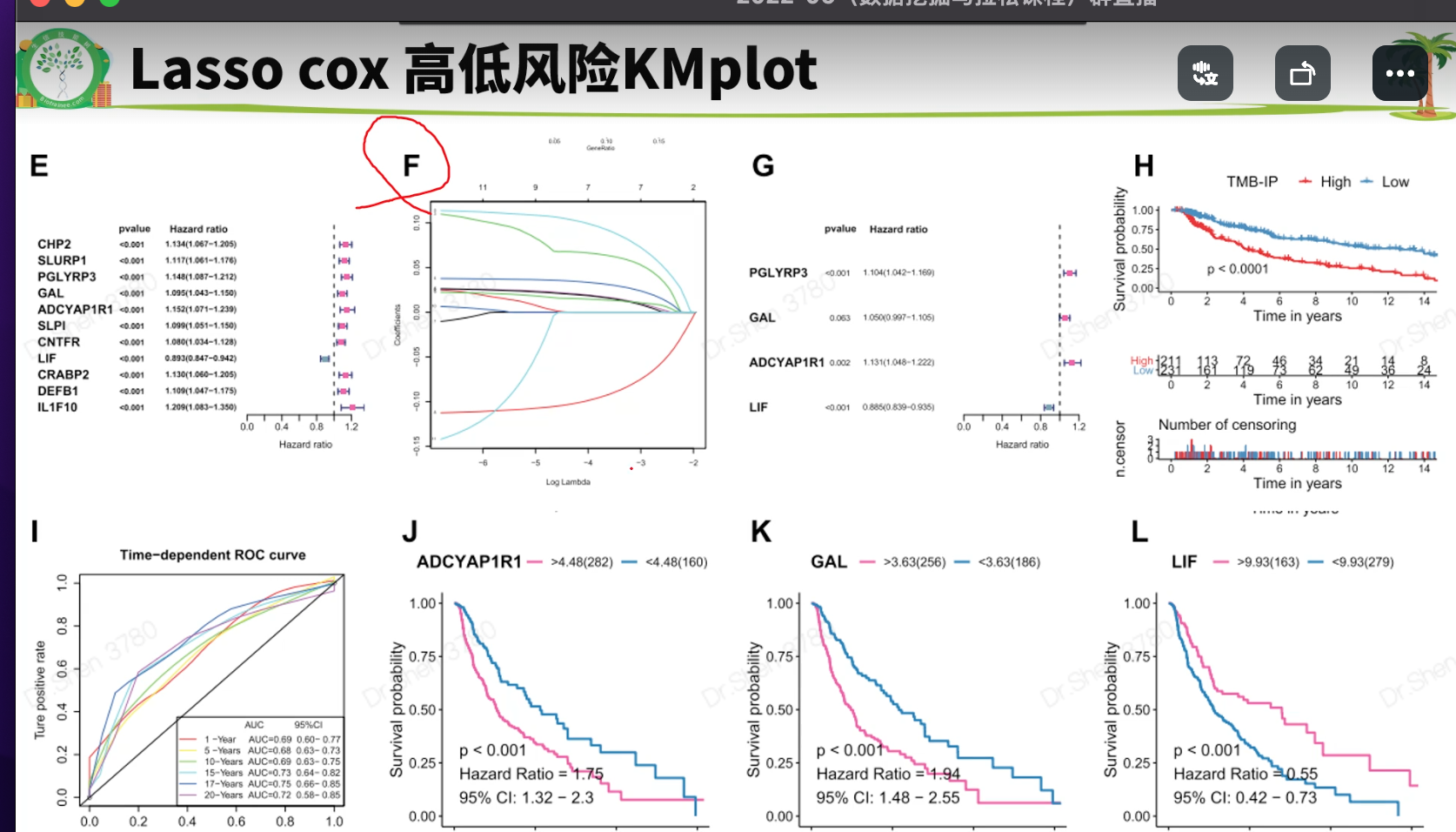
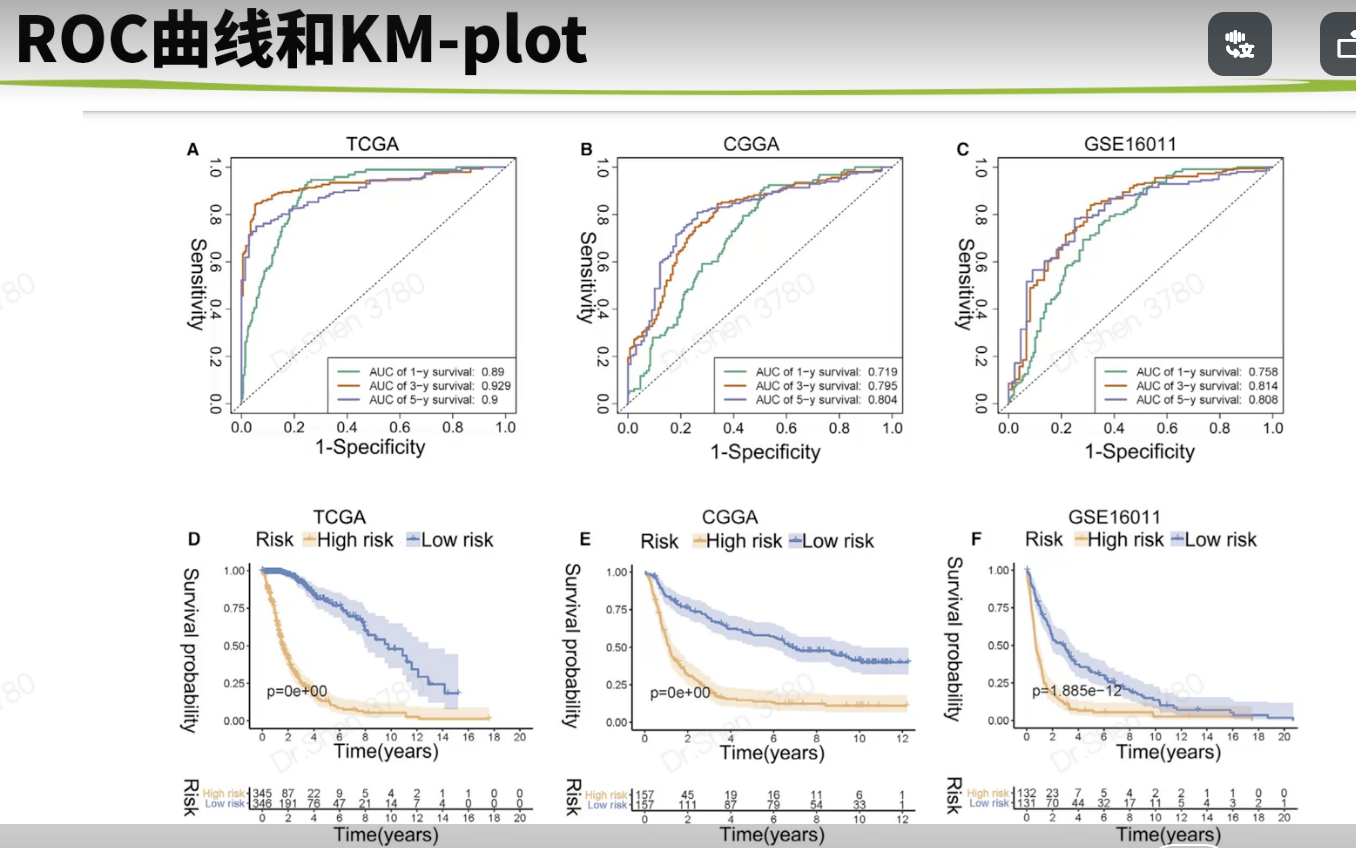
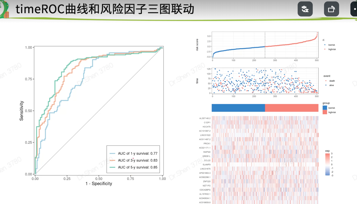
surv_cox_lassoER相关的基因endoplasmic reticulum stressgs = rio::import("GeneCards-SearchResults.csv")k = gs$`Relevance score`>=7;table(k)## k## FALSE TRUE## 6267 802gs = gs[k,]两种算法计算每个基因的p值,并取交集4个数据需要循环,先拿其中一个数据跑通,再把代码写入循环library(tinyarray)load("../1_data_pre/exp_surv1.Rdata")exp1 = exp1[rownames(exp1) %in% gs$`Gene Symbol`,]c1 = surv_cox(exp1,surv1,continuous = T)head(c1)## coef se z p HR HRse HRz## UBE2J2 1.4404365 0.13446765 10.712141 0.000000e+00 4.222539 0.5677949 5.675533## RER1 1.8780151 0.11813991 15.896534 0.000000e+00 6.540509 0.7726952 7.170369## ICMT 1.0621919 0.11658641 9.110770 0.000000e+00 2.892705 0.3372500 5.612170## PARK7 0.6545554 0.13911446 4.705157 2.536705e-06 1.924287 0.2676961 3.452746## H6PD 0.8217466 0.10642461 7.721396 1.154632e-14 2.274469 0.2420595 5.265107## FBXO6 0.9195681 0.08969749 10.251882 0.000000e+00 2.508207 0.2249799 6.703741## HRp HRCILL HRCIUL## UBE2J2 1.382573e-08 3.244252 5.495823## RER1 7.479573e-13 5.188606 8.244654## ICMT 1.998047e-08 2.301789 3.635320## PARK7 5.549107e-04 1.465060 2.527460## H6PD 1.401079e-07 1.846253 2.802004## FBXO6 2.031497e-11 2.103840 2.990295nrow(c1)## [1] 653k1 = surv_KM(exp1,surv1)head(k1) #p值实在太小,逼近0## UBE2J2 RER1 FBXO6 DDOST CDC42 SELENON## 0 0 0 0 0 0length(k1)## [1] 642g1 = intersect(rownames(c1),names(k1))head(g1)## [1] "UBE2J2" "RER1" "ICMT" "PARK7" "H6PD" "FBXO6"length(g1)## [1] 615循环load("../1_data_pre/exp_surv2.Rdata")load("../1_data_pre/exp_surv3.Rdata")load("../1_data_pre/exp_surv4.Rdata")exp = list(exp1,exp2,exp3,exp4)surv = list(surv1,surv2,surv3,surv4)g = list()for(i in 1:4){exp[[i]] = exp[[i]][rownames(exp[[i]]) %in% gs$`Gene Symbol`,]c1 = surv_cox(exp[[i]],surv[[i]],continuous = T)k = surv_KM(exp[[i]],surv[[i]])g[[i]] = intersect(rownames(c1),names(k))}names(g) = c("TCGA","CGGA_array","CGGA","GSE16011")sapply(g, length)## TCGA CGGA_array CGGA GSE16011## 615 413 551 335v_plot = draw_venn(g,"")ggplot2::ggsave(v_plot,filename = "venn.png")4个数据,两种算法p<0.05的基因取交集,得到195个基因,用于lasso回归g = intersect_all(g)length(g)## [1] 195lasso回归使用TCGA的数据构建模型library(survival)x = t(exp1[g,])y = data.matrix(Surv(surv1$time,surv1$event))library(glmnet)set.seed(10210)cvfit = cv.glmnet(x, y, family="cox")fit=glmnet(x, y, family = "cox")coef = coef(fit, s = cvfit$lambda.min)index = which(coef != 0)actCoef = coef[index]lassoGene = row.names(coef)[index]lassoGene## [1] "GPX7" "MR1" "SHISA5" "CP" "PPM1L" "DNAJB11"## [7] "SNCA" "ANXA5" "HFE" "EPM2A" "FKBP14" "BET1"## [13] "SERPINE1" "CASP2" "BAG1" "SIRT1" "DNAJB12" "ERLIN1"## [19] "CYP2E1" "CASP4" "SLN" "ERP27" "DDIT3" "ATP2A2"## [25] "ERP29" "MYH7" "CDKN3" "MAPK3" "MMP2" "NOL3"## [31] "BRCA1" "PRNP" "MX1" "RNF185" "SREBF2" "GLA"par(mfrow = c(1,2))plot(cvfit)plot(fit,xvar="lambda",label = F)逐步回归法library(My.stepwise)vl <- lassoGenedat = cbind(surv1,t(exp1[lassoGene,]))# My.stepwise.coxph(Time = "time",# Status = "event",# variable.list = vl,# data = dat)model = coxph(formula = Surv(time, event) ~ HFE + SHISA5 + BRCA1 + EPM2A +ERLIN1 + GPX7 + SLN + DNAJB11 + MMP2 + NOL3 + CP + ATP2A2 +GLA + MAPK3 + SREBF2 + CASP2 + SNCA + DDIT3 + BAG1 + ANXA5,data = dat)summary(model)$concordance## C se(C)## 0.865988496 0.009754695genes = names(model$coefficients);length(genes)## [1] 20library(survminer)ggforest(model,data = dat)ggsave("forest.png",width = 10,height = 8)计算风险评分dats = list(dat1 = cbind(surv1,t(exp1[genes,])),dat2 = cbind(surv2,t(exp2[genes,])),dat3 = cbind(surv3,t(exp3[genes,])),dat4 = cbind(surv4,t(exp4[genes,])))library(dplyr)survs = lapply(dats, function(x){fp = apply(x[,genes], 1,function(k)sum(model$coefficients * k)) #lasso回归模型的预测值就是线性加乘# x = x[,!(colnames(x)%in% genes)]x$fp = fpx$Risk = ifelse(x$fp<median(x$fp),"low","high")x$Risk = factor(x$Risk,levels = c("low","high"))return(x)})head(survs[[1]])## sample event _PATIENT time TYPE HFE## TCGA-06-0878-01A TCGA-06-0878-01A 0 TCGA-06-0878 218 GBM 2.3744248## TCGA-26-5135-01A TCGA-26-5135-01A 1 TCGA-26-5135 270 GBM 0.7702822## TCGA-06-5859-01A TCGA-06-5859-01A 0 TCGA-06-5859 139 GBM 2.5060929## TCGA-06-2563-01A TCGA-06-2563-01A 0 TCGA-06-2563 932 GBM 1.6765673## TCGA-41-2571-01A TCGA-41-2571-01A 1 TCGA-41-2571 26 GBM 0.7707545## TCGA-28-5207-01A TCGA-28-5207-01A 1 TCGA-28-5207 343 GBM 1.7947694## SHISA5 BRCA1 EPM2A ERLIN1 GPX7 SLN## TCGA-06-0878-01A 4.891004 1.929324 1.824520 2.963291 4.161208 3.2520898## TCGA-26-5135-01A 6.280796 1.535608 1.513929 2.027252 3.812280 3.3372085## TCGA-06-5859-01A 4.708155 3.118322 1.696385 2.702454 4.032823 3.6417199## TCGA-06-2563-01A 5.343170 1.324959 2.174987 2.690188 4.270150 0.9712369## TCGA-41-2571-01A 5.184783 1.082552 1.091940 1.892868 3.539653 2.8842578## TCGA-28-5207-01A 5.152544 1.958569 2.323285 2.802503 3.302680 0.9862039## DNAJB11 MMP2 NOL3 CP ATP2A2 GLA MAPK3## TCGA-06-0878-01A 4.489935 5.196985 3.954610 4.729828 4.931262 3.699737 4.639285## TCGA-26-5135-01A 3.934268 5.267932 3.521318 1.514229 5.054068 3.385206 5.064507## TCGA-06-5859-01A 3.360617 3.364497 2.896874 3.009394 4.516211 4.166703 4.214156## TCGA-06-2563-01A 3.828734 6.471976 1.931305 1.262133 4.879086 3.787763 4.527579## TCGA-41-2571-01A 3.083744 8.445514 3.889378 1.410165 4.753264 3.945768 4.887269## TCGA-28-5207-01A 3.558798 4.552452 2.013993 1.442487 4.530683 3.779798 4.950130## SREBF2 CASP2 SNCA DDIT3 BAG1 ANXA5 fp## TCGA-06-0878-01A 3.646879 3.056804 1.750464 5.599779 2.981576 7.777013 12.03249## TCGA-26-5135-01A 4.656178 2.837734 2.655945 5.330168 3.299911 7.067037 12.53646## TCGA-06-5859-01A 4.619645 2.662097 1.341060 5.621570 3.197839 6.306859 11.79212## TCGA-06-2563-01A 4.689714 3.175957 2.339013 4.388975 3.533318 7.995120 10.95347## TCGA-41-2571-01A 4.736130 3.262038 2.155570 5.840359 3.408114 6.413893 12.78245## TCGA-28-5207-01A 4.002934 3.147226 3.431305 7.208496 3.488568 7.653079 11.76648## Risk## TCGA-06-0878-01A high## TCGA-26-5135-01A high## TCGA-06-5859-01A high## TCGA-06-2563-01A high## TCGA-41-2571-01A high## TCGA-28-5207-01A highsave(model,genes,survs,file = "model_genes_survs.Rdata")survs里的每个数据都是由临床信息、建模基因的表达量、fp(预测值)、Risk(风险分组)构成,整理成了相同格式。timeROC曲线library(timeROC)result = list()p = list()for(i in 1:4){result[[i]] <-with(survs[[i]], timeROC(T=time,delta=event,marker=fp,cause=1,times=c(365,1095,1825),iid = TRUE))dat = data.frame(fpr = as.numeric(result[[i]]$FP),tpr = as.numeric(result[[i]]$TP),time = rep(as.factor(c(365,1095,1825)),each = nrow(result[[i]]$TP)))library(ggplot2)p[[i]] = ggplot() +geom_line(data = dat,aes(x = fpr, y = tpr,color = time),size = 1) +scale_color_manual(name = NULL,values = c("#92C5DE", "#F4A582", "#66C2A5"),labels = paste0("AUC of ",c(1,3,5),"-y survival: ",format(round(result[[i]]$AUC,2),nsmall = 2)))+geom_line(aes(x=c(0,1),y=c(0,1)),color = "grey")+theme_bw()+theme(panel.grid = element_blank(),legend.background = element_rect(linetype = 1, size = 0.2, colour = "black"),legend.position = c(0.765,0.125))+scale_x_continuous(expand = c(0.005,0.005))+scale_y_continuous(expand = c(0.005,0.005))+labs(x = "1 - Specificity",y = "Sensitivity")+coord_fixed()}library(patchwork)wrap_plots(p)ggsave("time_ROC.png",height = 10,width = 10)高低风险KM_plotlibrary(survival)library(survminer)corhorts = c("TCGA","CGGA_array","CGGA","GSE16011")splots = list()for(i in 1:4){x = survs[[i]]sfit1 = survfit(Surv(time, event) ~ Risk, data = x)splots[[i]] = ggsurvplot(sfit1, pval = TRUE, palette = "jco",data = x, legend = c(0.8, 0.8), title =corhorts[[i]],risk.table = T)}png("survs.png",height = 800,width = 800)arrange_ggsurvplots(splots,nrow = 2)dev.off()## png## 2### 三图联动有缺失time和event的样本前面没有去掉,画图会出NA,但是动了前面结果就会变化很大,猜测作者是只在画图时去掉了,不参考他的做法,你自己做时整理临床信息时就去掉,这里就不会出NA了。source("risk_plot.R")risk_plot(survs[[1]],genes)risk_plot(survs[[2]],genes)risk_plot(survs[[3]],genes)risk_plot(survs[[4]],genes)
for循环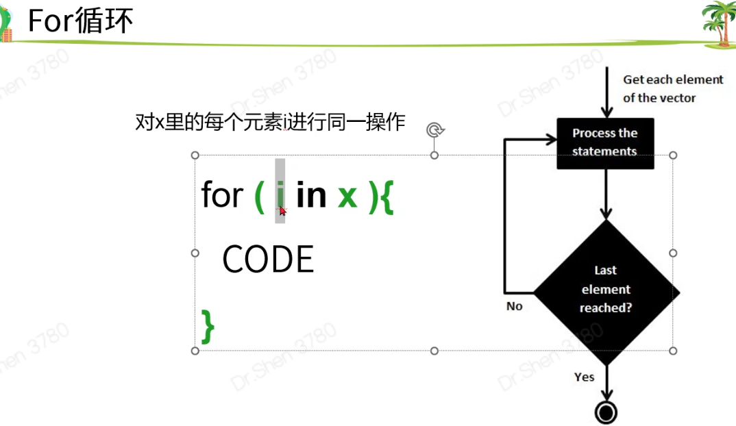
逐步回归法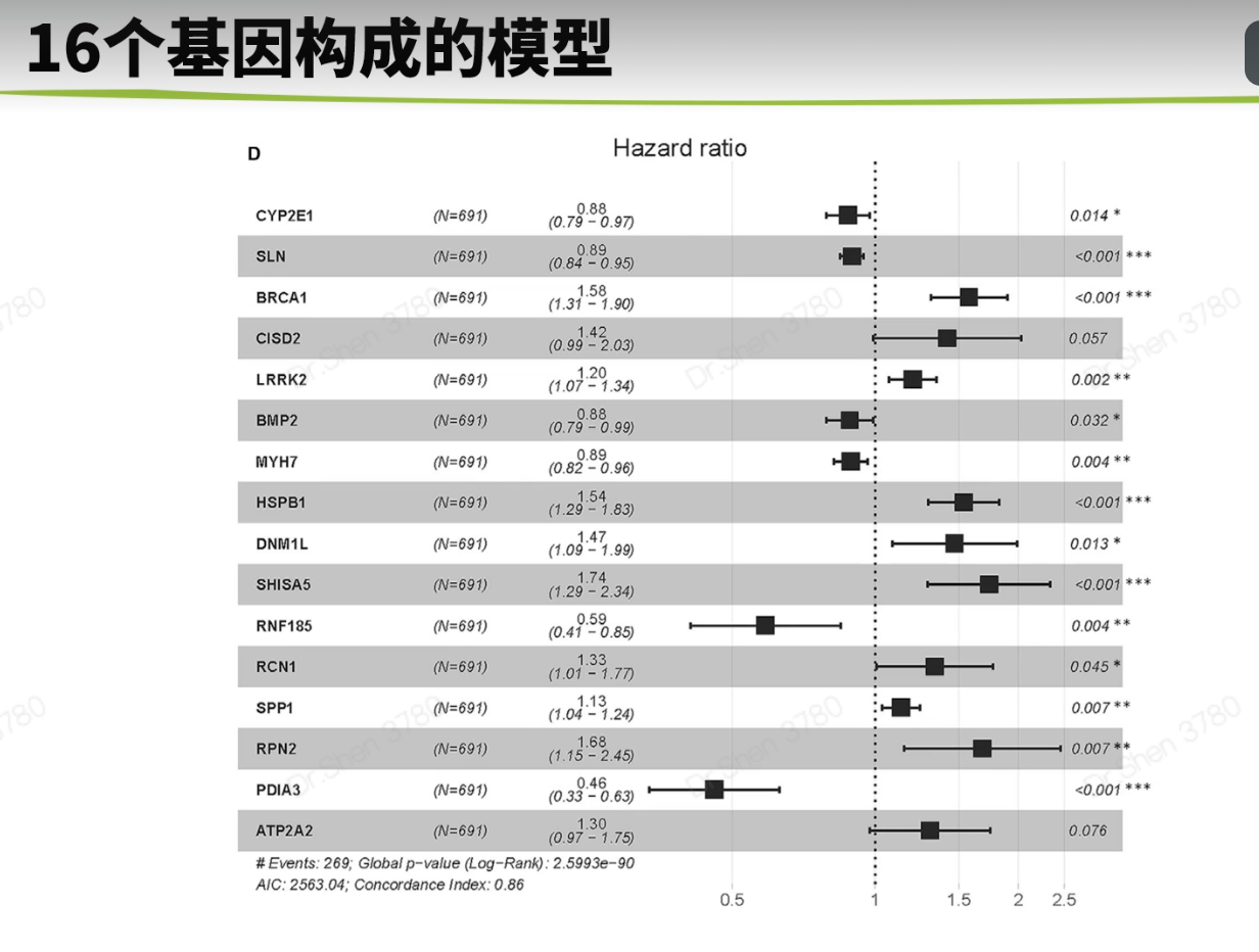
三图联动
三张图的顺序都一样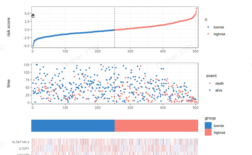
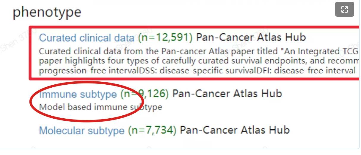
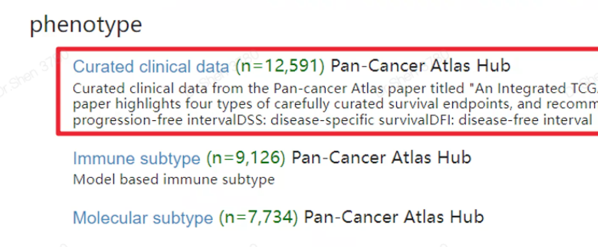
 免疫亚型
免疫亚型
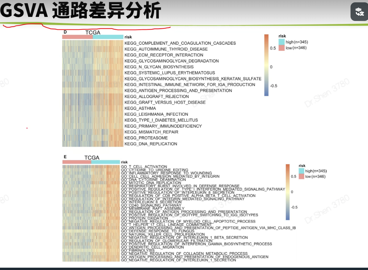
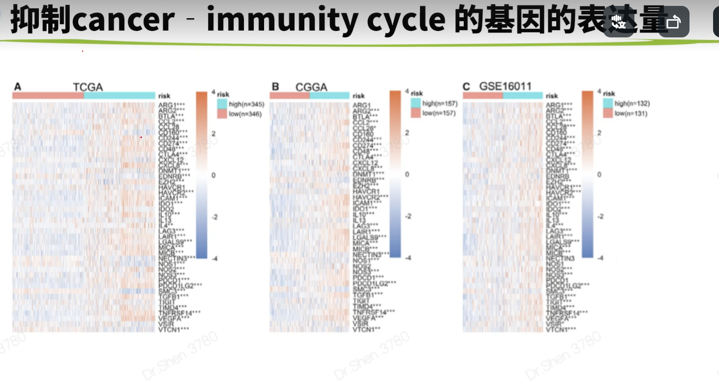
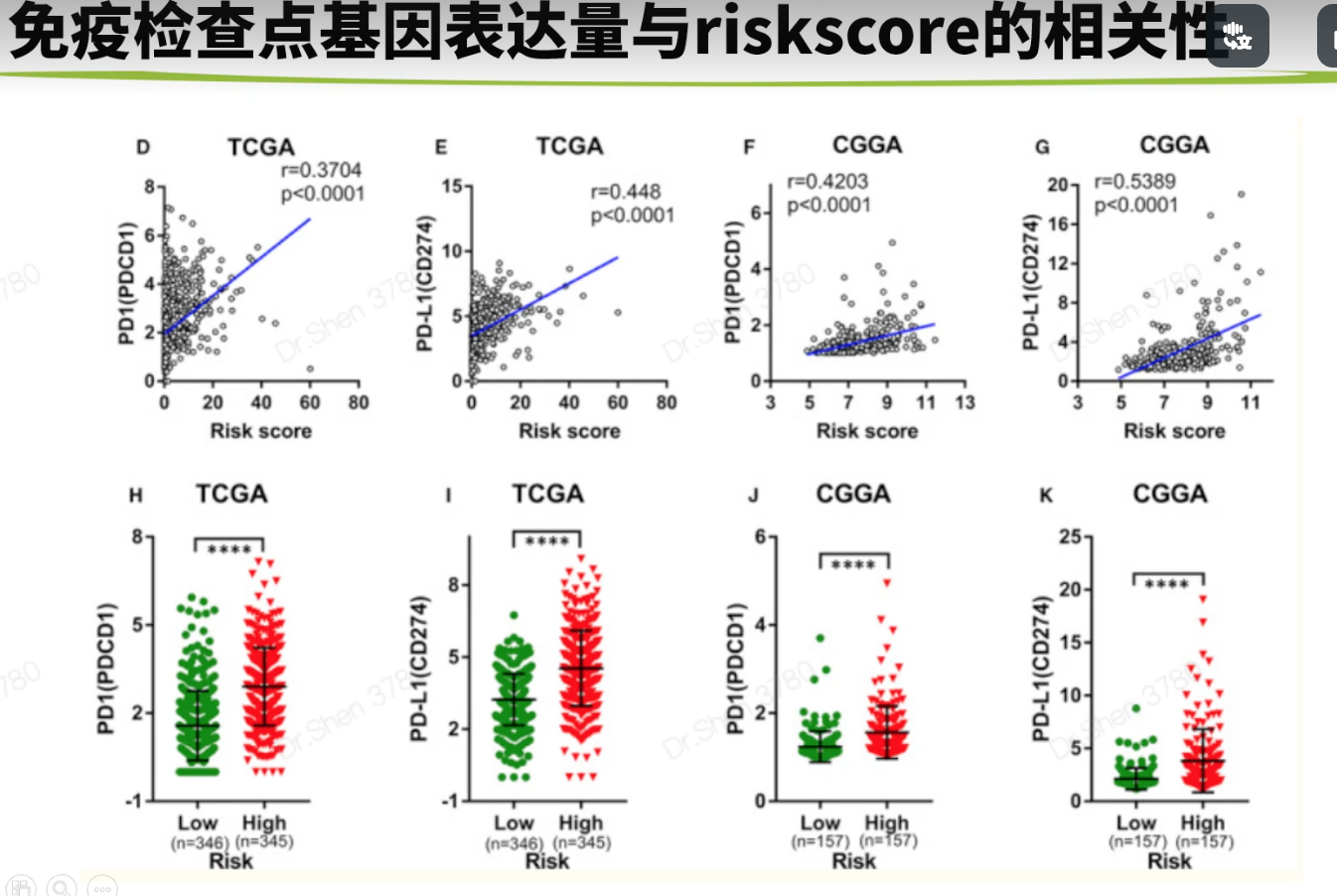
免疫相关的分析生信技能树1.抑制cancer‐immunity cycle 的基因http://biocc.hrbmu.edu.cn/TIP/index.jsprm(list = ls())library(tinyarray)tip = read.delim("TIP_genes.txt",header = T)nrow(tip)## [1] 273head(tip)## GeneSymbol Steps Direction ImmuneCellType## 1 IL10 1 positive Multiple## 2 TGFB1 1 positive Multiple## 3 HMGB1 1 positive Multiple## 4 ANXA1 1 positive Multiple## 5 CALR 1 positive Multiple## 6 CXCL10 1 positive Multiplegs = tip$GeneSymbol[tip$Direction =="negative"];length(gs)## [1] 54load("../1_data_pre/exp_surv1.Rdata")load("../1_data_pre/exp_surv2.Rdata")load("../1_data_pre/exp_surv3.Rdata")load("../1_data_pre/exp_surv4.Rdata")load("../2_model/model_genes_survs.Rdata")exps = list(exp1,exp2,exp3,exp4)#i = 1p1 = list()corhorts = c("TCGA","CGGA_array","CGGA","GSE16011")for(i in 1:4){n = exps[[i]][rownames(exps[[i]])%in% gs,]n = n[,order(survs[[i]]$fp)]g = sort(survs[[i]]$Risk)rn = apply(n,1,function(x){#x = n[1,]p = wilcox.test(x~g)$p.valuej = ifelse(p<=0.001,"***",ifelse(p<=0.01,"**",ifelse(p<=0.05,"*","")))return(j)})rownames(n) = paste0(rownames(n),rn)p1[[i]] =draw_heatmap(n,g,cluster_cols = F,main = corhorts[[i]],show_rownames = T)}library(patchwork)wrap_plots(p1)箱线图g4 = c("VEGFA","TGFB1","CD95L","CD70")p2 = list()library(ggplot2)for(i in 1:4){p2[[i]] = draw_boxplot(exps[[i]][rownames(exps[[i]])%in% g4,],survs[[i]]$Risk,sort = F)+ggtitle(corhorts[[i]])+theme(plot.title = element_text(hjust = 0.5))}library(ggplot2)wrap_plots(p2) + plot_layout(guides = "collect") &theme(legend.position='right')没有找到CD95L基因。这里仅作例子,自己文章中用到的重要基因,可以查查别名。2.免疫细胞丰度用ssgsea方法。mmc3.xlsx出自这篇文章的TableS6:https://www.sciencedirect.com/science/article/pii/S2211124716317090geneset = rio::import("mmc3.xlsx",skip = 2)geneset = split(geneset$Metagene,geneset$`Cell type`)lapply(geneset[1:3], head)## $`Activated B cell`## [1] "ADAM28" "CD180" "CD79B" "BLK" "CD19" "MS4A1"#### $`Activated CD4 T cell`## [1] "AIM2" "BIRC3" "BRIP1" "CCL20" "CCL4" "CCL5"#### $`Activated CD8 T cell`## [1] "ADRM1" "AHSA1" "C1GALT1C1" "CCT6B" "CD37" "CD3D"library(GSVA)f = "ssgsea_result.Rdata"if(!file.exists(f)){p = list()for(i in 1:4){#i = 1re <- gsva(exps[[i]], geneset, method="ssgsea",mx.diff=FALSE, verbose=FALSE)p[[i]] = draw_boxplot(re,survs[[i]]$Risk)+ggtitle(corhorts[[i]])+theme(plot.title = element_text(hjust = 0.5))+theme(plot.margin=unit(c(1,3,1,1),'lines')) #调整边距}save(re,p,file = f)}load(f)wrap_plots(p)+ plot_layout(guides = "collect") &theme(legend.position='right')免疫亚型#devtools::install_github("Gibbsdavidl/ImmuneSubtypeClassifier")library(ImmuneSubtypeClassifier)f = "immu_res.Rdata"if(!file.exists(f)){res = list()for(i in 1:4){a <- callEnsemble(X = exps[[i]], geneids = 'symbol')[,1:2]a$corhort = corhorts[[i]]a$Risk = survs[[i]]$Riskres[[i]] = a}save(res,file = f)}load(f)我检查了一下这个方法和xena整理结果是否一致a1 = res[[1]]head(a1)## SampleIDs BestCall corhort Risk## 1 TCGA-06-0878-01A 4 TCGA high## 2 TCGA-26-5135-01A 4 TCGA high## 3 TCGA-06-5859-01A 4 TCGA high## 4 TCGA-06-2563-01A 4 TCGA high## 5 TCGA-41-2571-01A 4 TCGA high## 6 TCGA-28-5207-01A 4 TCGA higha1$SampleIDs = str_sub(a1$SampleIDs,1,15)a2 = read.delim("Subtype_Immune_Model_Based.txt.gz")head(a2)## sample Subtype_Immune_Model_Based## 1 TCGA-A5-A0GI-01 Wound Healing (Immune C1)## 2 TCGA-S9-A7J2-01 Immunologically Quiet (Immune C5)## 3 TCGA-EK-A2RE-01 IFN-gamma Dominant (Immune C2)## 4 TCGA-D5-5538-01 IFN-gamma Dominant (Immune C2)## 5 TCGA-F4-6854-01 Wound Healing (Immune C1)## 6 TCGA-AX-A2H7-01 Wound Healing (Immune C1)table(a1$SampleIDs %in% a2$sample)#### FALSE TRUE## 34 657a = merge(a1,a2,by.x = "SampleIDs",by.y = "sample")a$check = str_extract(a$Subtype_Immune_Model_Based,"\\d")table(a$check==a$BestCall)#### FALSE TRUE## 59 598大部分一致吧。但还是有一些出入的res2 = do.call(rbind,res)head(res2)## SampleIDs BestCall corhort Risk## 1 TCGA-06-0878-01A 4 TCGA high## 2 TCGA-26-5135-01A 4 TCGA high## 3 TCGA-06-5859-01A 4 TCGA high## 4 TCGA-06-2563-01A 4 TCGA high## 5 TCGA-41-2571-01A 4 TCGA high## 6 TCGA-28-5207-01A 4 TCGA highres2$BestCall = factor(paste0("C",res2$BestCall))library(dplyr)dat2 <- res2 %>%group_by(corhort,Risk, BestCall) %>%summarise(count = n())library(paletteer)pb = ggplot() + geom_bar(data =dat2, aes(x = Risk, y = count, fill = BestCall),stat = "identity",position = "fill")+theme_classic()+scale_fill_paletteer_d("RColorBrewer::Set2")+labs(x = "Risk",y = "Percentage")+facet_wrap(~corhort,nrow = 1)pb免疫检查点基因https://www.ncbi.nlm.nih.gov/pmc/articles/PMC7786136/# 别名 B7-H3 是CD276;PD-L1是CD274;PD-1是PDCD1,PDCD1LG2是PD-L2tmp = readLines("immune_checkpoint.txt")genes = str_split(tmp,", ")[[1]]sapply(exps, function(x){genes[!(genes %in% rownames(x))]})## [[1]]## character(0)#### [[2]]## character(0)#### [[3]]## [1] "BTNL2" "IDO2" "KIR3DL1"#### [[4]]## [1] "IDO2"pi = list()for(i in 1:4){n = exps[[i]][rownames(exps[[i]])%in% genes,]n = n[,order(survs[[i]]$fp)]g = sort(survs[[i]]$Risk)rn = apply(n,1,function(x){#x = n[1,]p = wilcox.test(x~g)$p.valuej = ifelse(p<=0.001,"***",ifelse(p<=0.01,"**",ifelse(p<=0.05,"*","")))return(j)})rownames(n) = paste0(rownames(n),rn)pi[[i]] =draw_heatmap(n,g,cluster_cols = F,main = corhorts[[i]],show_rownames = T)}library(patchwork)wrap_plots(pi)相关性与箱线图#i = 1library(ggpubr)pc = list()for(i in 1:4){dat = data.frame(PDCD1 = exps[[i]]["PDCD1",],CD274 = exps[[i]]["CD274",],risk_score = survs[[i]]$fp,Risk = survs[[i]]$Risk)p1 = ggscatter( dat,y = "PDCD1", x = "risk_score",xlab = "Risk score",size =1,color = "#1d4a9d",add = "reg.line",add.params = list(color = "red"))+stat_cor(label.y = 5)p2 = ggscatter( dat,y = "CD274", x = "risk_score",xlab = "Risk score",size =1,color = "#1d4a9d",add = "reg.line",add.params = list(color = "red"),title = corhorts[[i]])+stat_cor(label.y = 5)p3 = draw_boxplot(t(dat[,1:2]),dat$Risk)pc[[i]] = list(p1,p2,p3)}wrap_plots(c(pc[[1]],pc[[2]],pc[[3]],pc[[4]]),nrow = 2)
文献4

若有收获,就点个赞吧
0 人点赞
