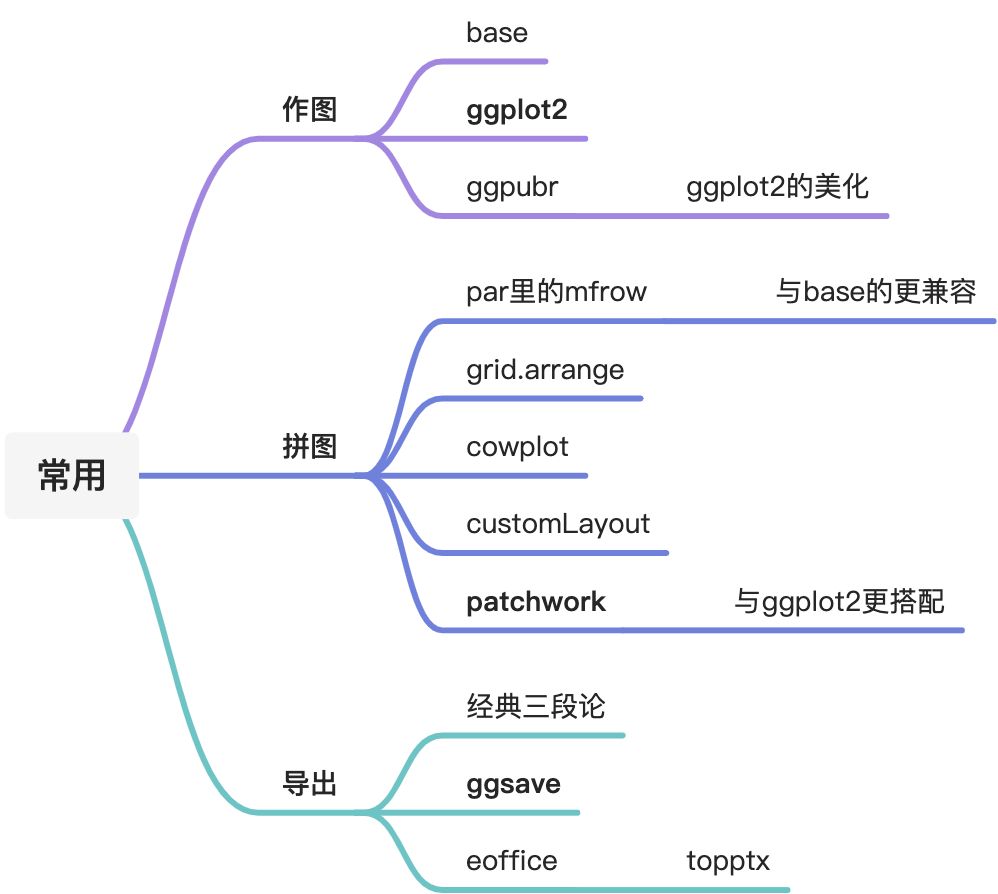
1、基础包—绘图函数
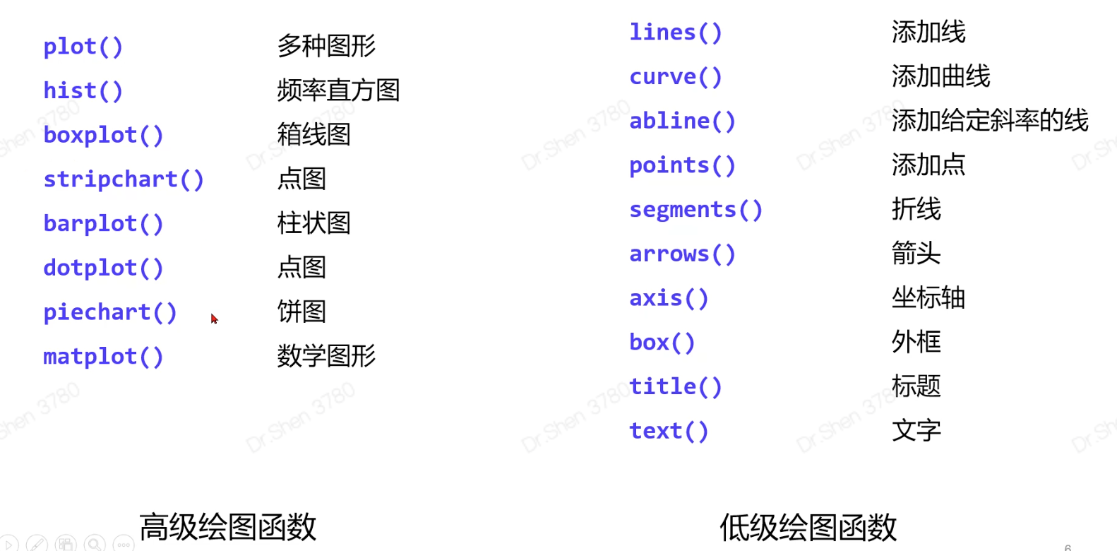
*高级:直接出图片;低级:需要以图片作为基础
#1.基础包 ,了解plot(iris[,1],iris[,3],col = iris[,5]) #横坐标,纵坐标,颜色text(6.5,4, labels = 'hello')# 某坐标添加文字dev.off() #关闭画板
2、ggplot2与ggpubr
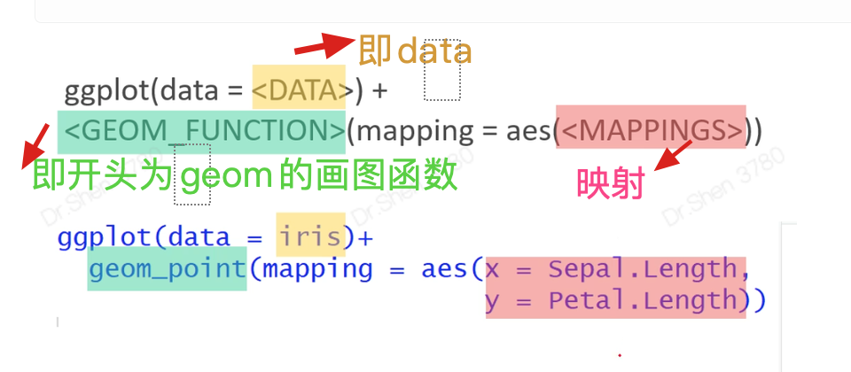
2.1作图数据、横纵坐标
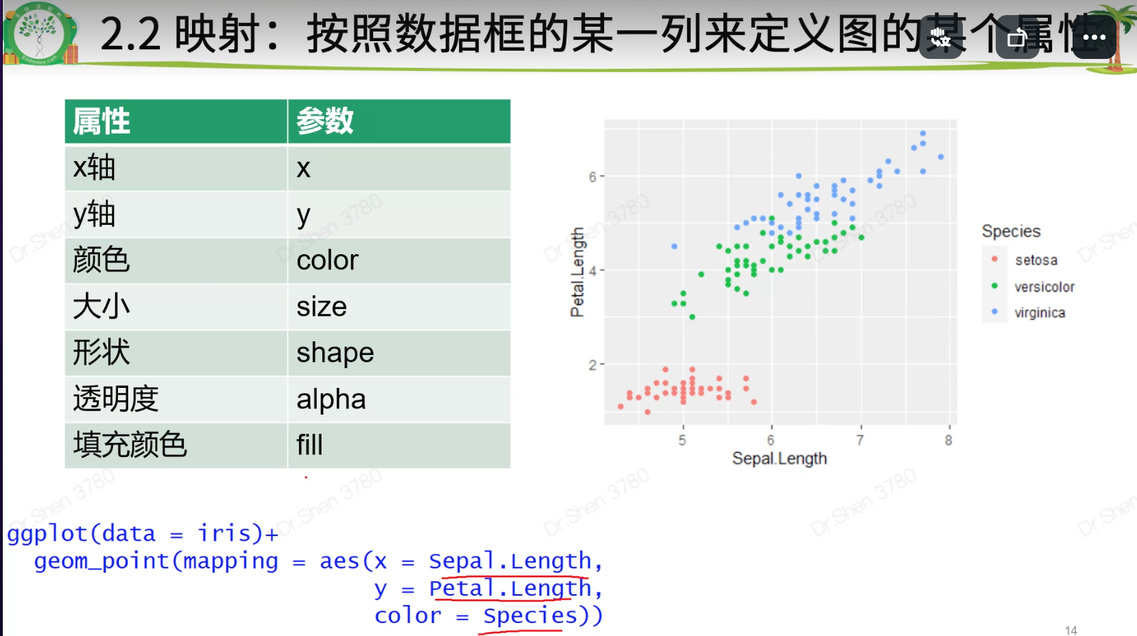
ggplot(data = <DATA>)+<geom_point>(mapping = aes(<MAPPINGS>))<>:表示代替内容特殊语法:列名不带引号,行末写加号用“+”连接不同的函数
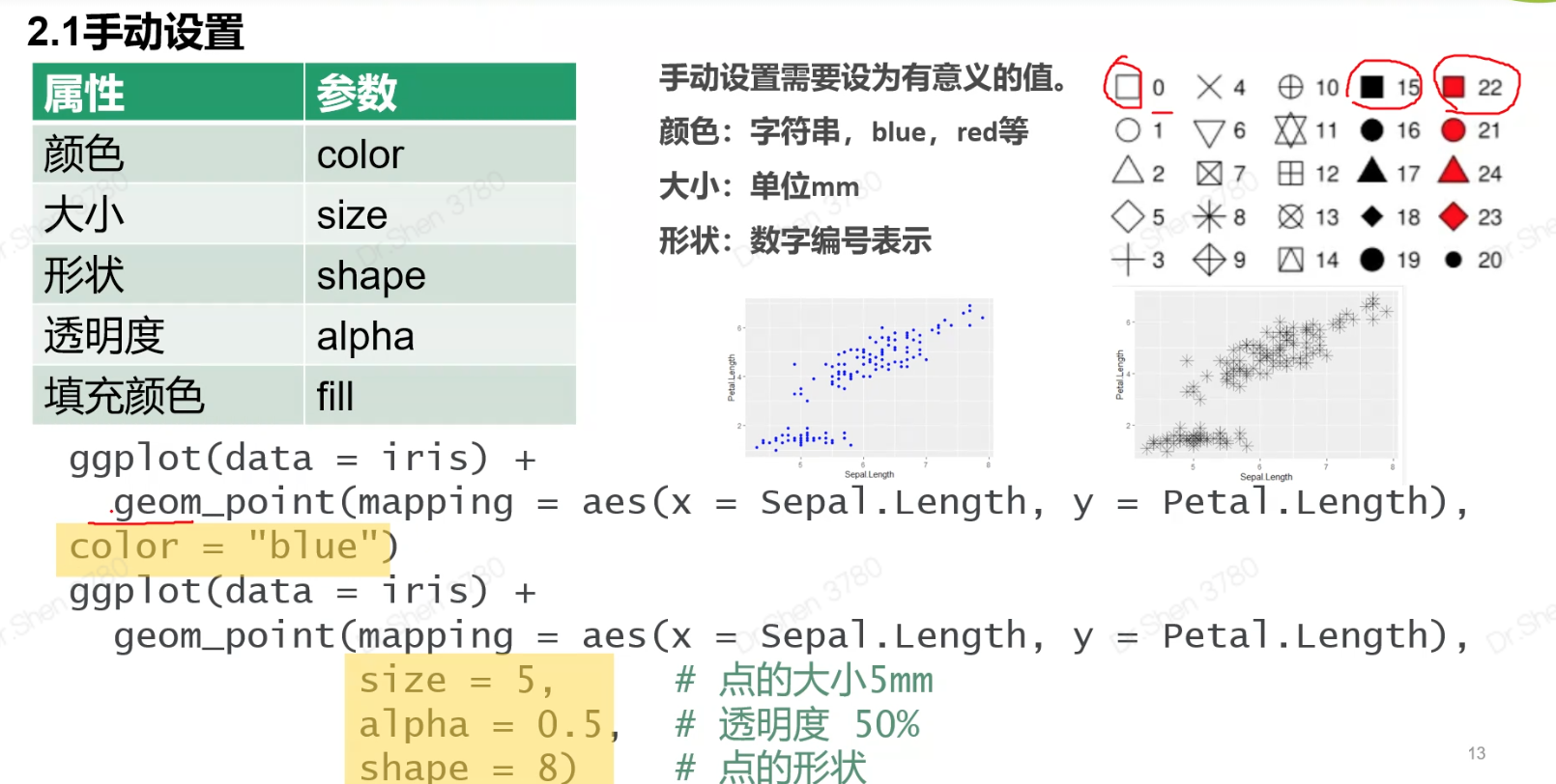
2.2属性设置
映射
映射和手动设置的区别:
映射是根据数据的某一列的内容分配颜色。 color = Species
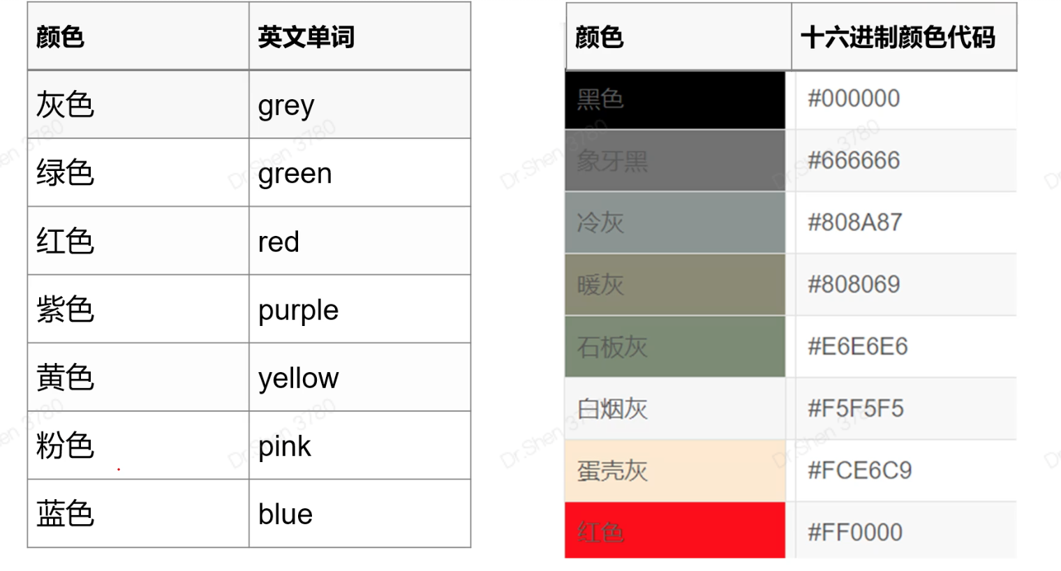
手动设置:把图形设置为一个或几个颜色,与数据内容无关。 color = “blue”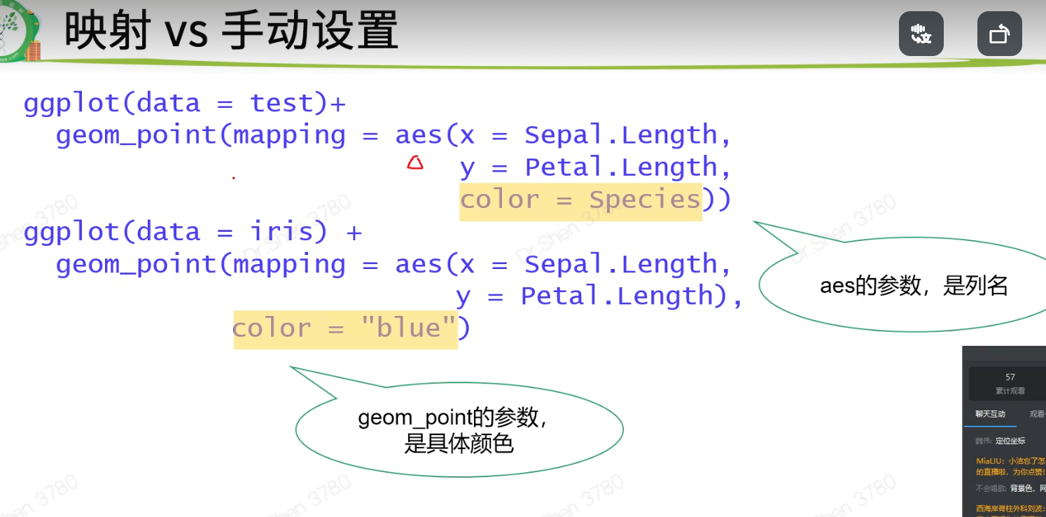
填充

2.3分面
三分面和双分面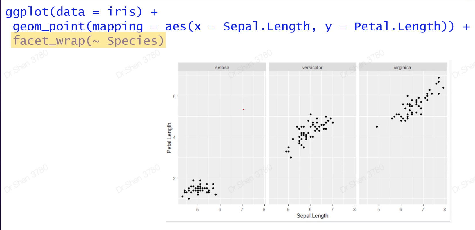
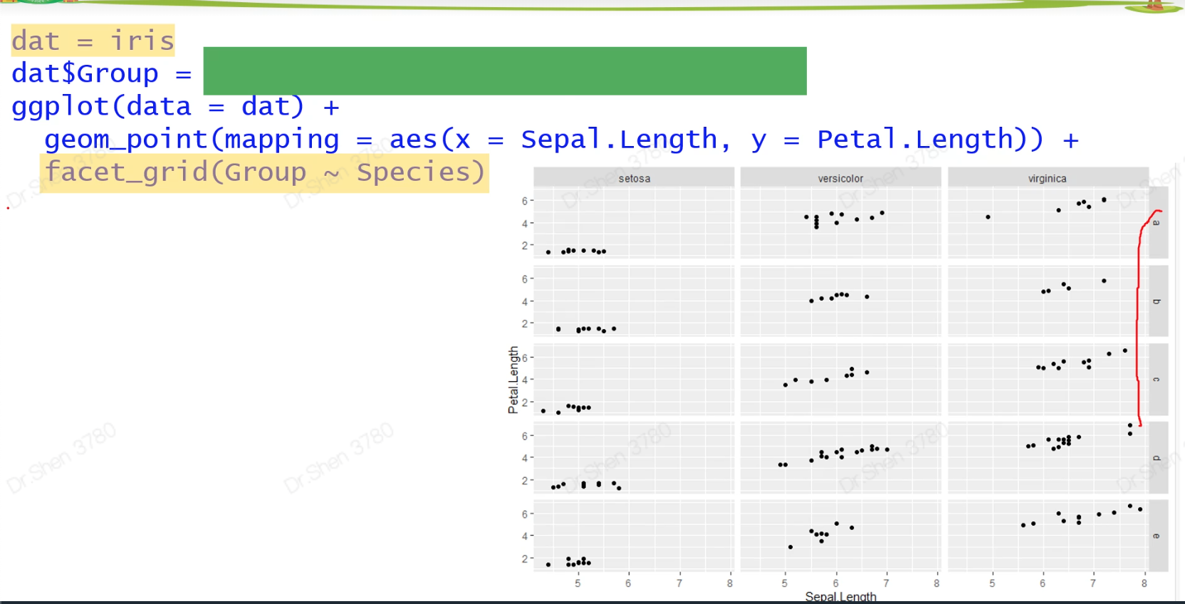
认识函数:sample(letters[1:5],150,replace = T)
上述涉及的代码
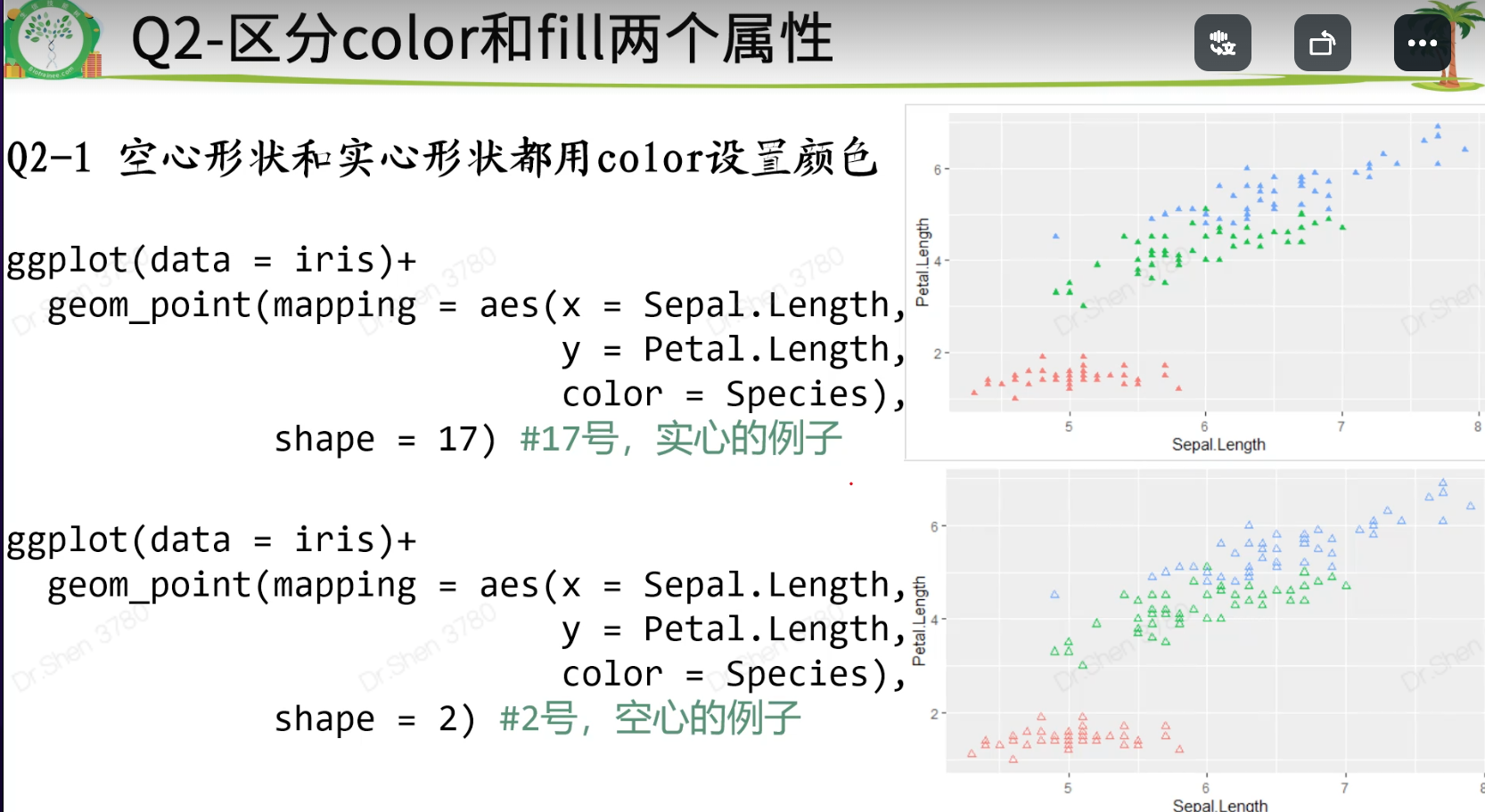
library(ggplot2)#1.入门级绘图模板:作图数据,横纵坐标ggplot(data = iris)+geom_point(mapping = aes(x = Sepal.Length,y = Petal.Length))#2.属性设置(颜色、大小、透明度、点的形状,线型等)#2.1 手动设置,需要设置为有意义的值ggplot(data = iris) +geom_point(mapping = aes(x = Sepal.Length,y = Petal.Length),color = "blue")ggplot(data = iris) +geom_point(mapping = aes(x = Sepal.Length, y = Petal.Length),size = 5, # 点的大小5mmalpha = 0.5, # 透明度 50%shape = 8) # 点的形状#2.2 映射:按照数据框的某一列来定义图的某个属性ggplot(data = iris)+geom_point(mapping = aes(x = Sepal.Length,y = Petal.Length,color = Species))#映射VS 手动设置ggplot(data = iris)+geom_point(mapping = aes(x = Sepal.Length,y = Petal.Length),color = "blue")## Q1 自行指定映射的具体颜色ggplot(data = iris)+geom_point(mapping = aes(x = Sepal.Length,y = Petal.Length,color = Species))+scale_color_manual(values = c("blue","grey","red"))## Q2 区分color和fill两个属性### Q2-1 空心形状和实心形状都用color设置颜色ggplot(data = iris)+geom_point(mapping = aes(x = Sepal.Length,y = Petal.Length,color = Species),shape = 17) #17号,实心的例子ggplot(data = iris)+geom_point(mapping = aes(x = Sepal.Length,y = Petal.Length,color = Species),shape = 2) #2号,空心的例子### Q2-2 既有边框又有内心的,才需要color和fill两个参数ggplot(data = iris)+geom_point(mapping = aes(x = Sepal.Length,y = Petal.Length,color = Species),shape = 24,fill = "black") #24号,双色的例子#3.分面ggplot(data = iris) +geom_point(mapping = aes(x = Sepal.Length, y = Petal.Length)) +facet_wrap(~ Species) #3张子图#双分面dat = iris #注意避免修改内置数据dat$Group = sample(letters[1:5],150,replace = T)ggplot(data = dat) +geom_point(mapping = aes(x = Sepal.Length, y = Petal.Length)) +facet_grid(Group ~ Species) #横纵均分面,有重复值,有限#认识sample函数sample(letters[1:5],3)#带有随机性sample(letters[1:5],6)#有范围的取样,6大于5,故会报错sample(letters[1:5],6,replace = T)#添加上replace = T,则可循环
2.4几何对象
geom_xxx()画出单个几何对象,几何对象可叠加
#4.几何对象#局部设置(仅对当前图层有效)和全局设置(对所有图层有效)#geom_xxx()画出单个几何对象,几何对象可叠加ggplot(data = iris) +geom_smooth(mapping = aes(x = Sepal.Length,y = Petal.Length))+geom_point(mapping = aes(x = Sepal.Length,y = Petal.Length))#简化上述代码,如下ggplot(data = iris,mapping = aes(x = Sepal.Length, y = Petal.Length))+geom_smooth()+geom_point()
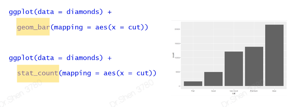
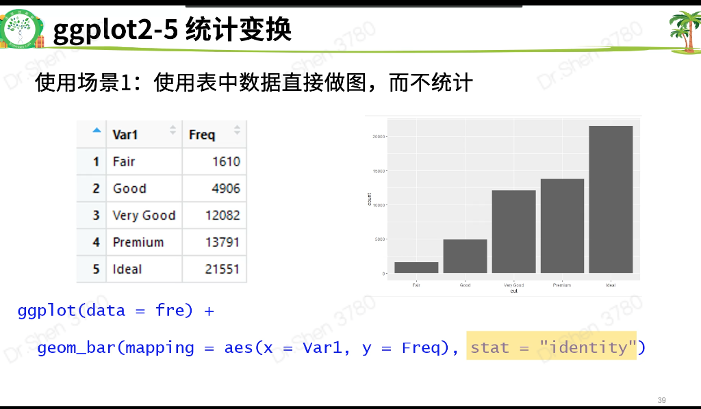
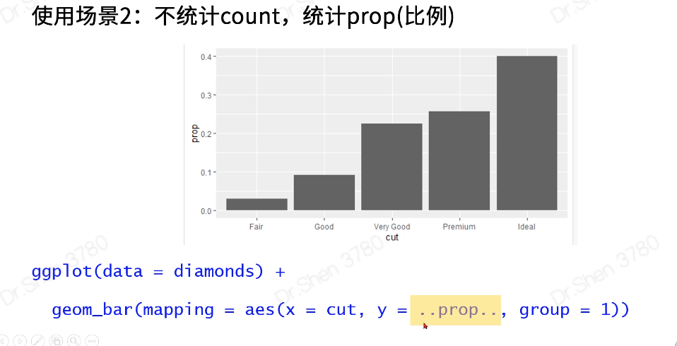
2.5统计变换
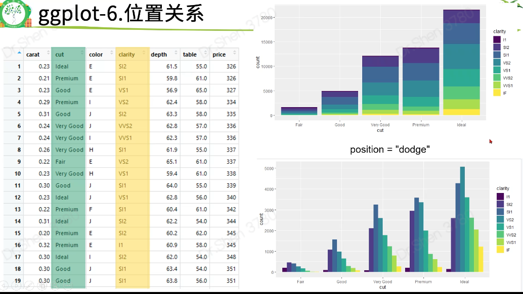
2.6位置关系
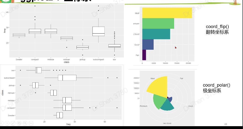
2.7坐标系
涉及代码
#5.统计变换-直方图View(diamonds)table(diamonds$cut)#画条形图,了解。自动生成yggplot(data = diamonds) +geom_bar(mapping = aes(x = cut))#展示数据,了解ggplot(data = diamonds) +stat_count(mapping = aes(x = cut))#统计变换使用场景#5.1.不统计,数据直接做图fre = as.data.frame(table(diamonds$cut))freggplot(data = fre) +geom_bar(mapping = aes(x = Var1, y = Freq), stat = "identity")#5.2count改为propggplot(data = diamonds) +geom_bar(mapping = aes(x = cut, y = ..prop.., group = 1))#6.位置关系# 6.1抖动的点图 ,geom_jitterggplot(data = iris,mapping = aes(x = Species,y = Sepal.Width,fill = Species)) +geom_boxplot()+geom_point()ggplot(data = iris,mapping = aes(x = Species,y = Sepal.Width,fill = Species)) +geom_boxplot()+geom_jitter()# 6.2堆叠直方图ggplot(data = diamonds) +geom_bar(mapping = aes(x = cut,fill=clarity))# 6.3 并列直方图ggplot(data = diamonds) +geom_bar(mapping = aes(x = cut, fill = clarity), position = "dodge")#7.坐标系#翻转coord_flip()ggplot(data = mpg, mapping = aes(x = class, y = hwy)) +geom_boxplot() +coord_flip()#极坐标系coord_polar()bar <- ggplot(data = diamonds) +geom_bar(mapping = aes(x = cut, fill = cut),width = 1) +theme(aspect.ratio = 1) +labs(x = NULL, y = NULL)barbar + coord_flip() #翻转坐标系bar + coord_polar()#极坐标系
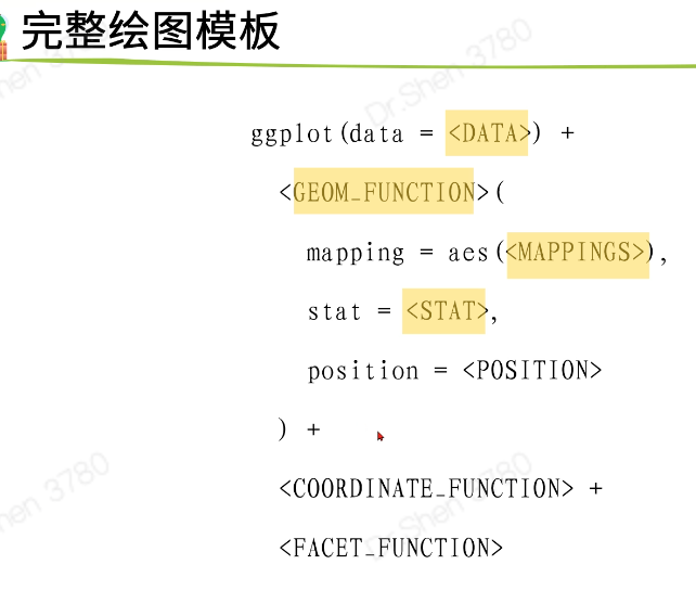
绘图模板
3、ggpubr
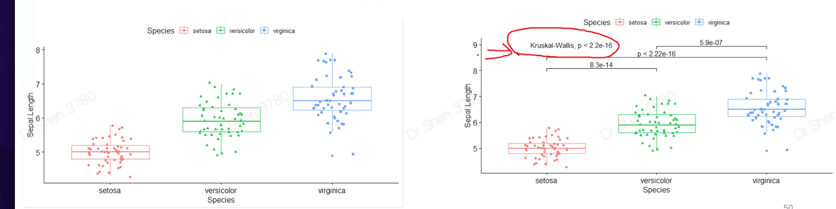
# ggpubr 搜代码直接用,不需要系统学习# sthda上有大量ggpubr出的图library(ggpubr)ggscatter(iris,x="Sepal.Length",y="Petal.Length",color="Species")theme_bw() #可将背景消除p <- ggboxplot(iris, x = "Species",y = "Sepal.Length",color = "Species",shape = "Species",add = "jitter")pmy_comparisons <- list( c("setosa", "versicolor"),c("setosa", "virginica"),c("versicolor", "virginica") )p + stat_compare_means(comparisons = my_comparisons)+ # Add pairwise comparisons p-valuestat_compare_means(label.y = 9)
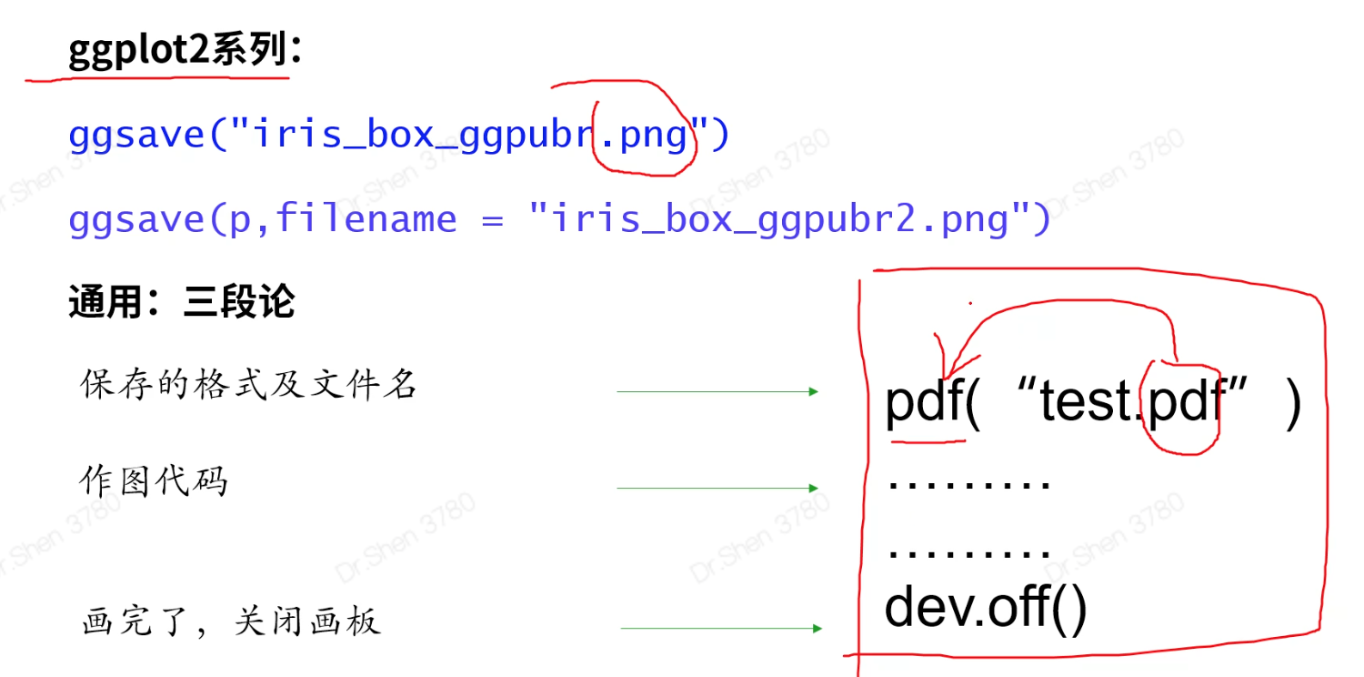
图片的保存与导出
三种方式#1.ggplot2,图片的后缀很重要ggsave(“名称.png”)ggsave(p,filename=“名称.png”)#2.三段论#3.eofficelibrary(eoffice)topptx(p,“名称.pptx”)#图片保存的三种方法#1.基础包作图的保存pdf("iris_box_ggpubr.pdf")boxplot(iris[,1]~iris[,5])text(6.5,4, labels = 'hello')dev.off()#2.ggplot系列图(包括ggpubr)通用的简便保存 ggsavep <- ggboxplot(iris, x = "Species",y = "Sepal.Length",color = "Species",shape = "Species",add = "jitter")ggsave(p,filename = "iris_box_ggpubr.png",width = 12,height = 9)#3.eoffice包 导出为ppt,全部元素都是可编辑模式library(eoffice)topptx(p,"iris_box_ggpubr.pptx")#https://mp.weixin.qq.com/s/p7LLLvzR5LPgHhuRGhYQBQ
拼图

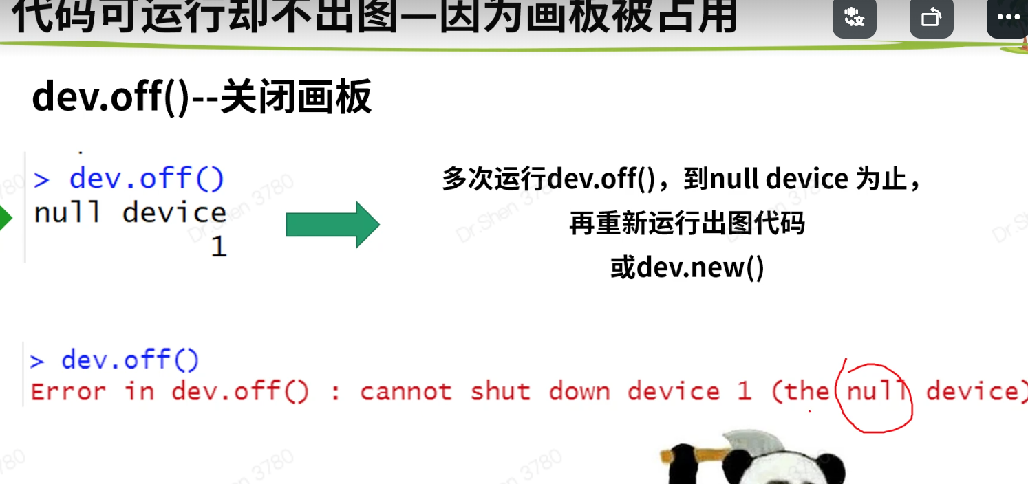
关闭画板:dev.off()
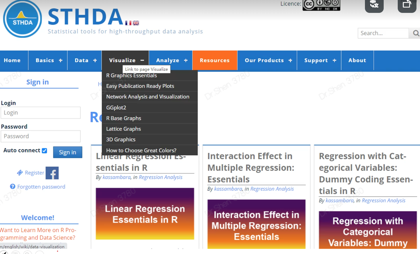
画图代码来源:STHDA
画图R包:ggstatsplot
library(ggstatsplot)
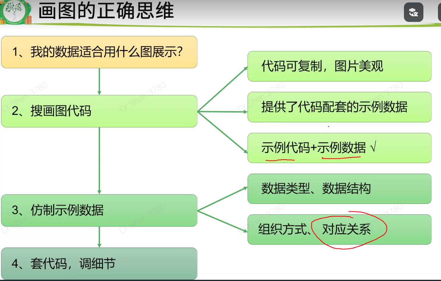
画图的思维
作业
# 6-1# 1.加载test.Rdata,分别test的以a和b列作为横纵坐标,change列映射颜色,画点图。load("test.Rdata")ggplot(data = test)+geom_point(mapping = aes(x = a,y = b,color = change))# 2.尝试修改点的颜色为暗绿色(darkgreen)、灰色、红色ggplot(data = test)+geom_point(mapping = aes(x = a,y = b,color = change))+scale_color_manual(values = c("darkgreen","grey","red"))# 1.尝试写出下图的代码,小提琴图ggplot(iris,aes(x = Sepal.Width,y = Species))+geom_violin(aes(fill = Species)) +geom_boxplot()+geom_jitter(aes(shape=Species))ggplot(data = iris,mapping = aes(x = Species,y = Sepal.Width))+geom_violin(aes(fill = Species))+geom_boxplot()+geom_jitter(aes(shape = Species))+coord_flip()# 6-3# 任意作3张ggplot2图ggplot(data = iris) +geom_smooth(mapping = aes(x = Sepal.Length,y = Petal.Length),color = "blue")# 1.探索labs() 函数如何使用#1.1 设置标题、副标题、引用ggplot(data = iris) +geom_smooth(mapping = aes(x = Sepal.Length,y = Petal.Length),color = "blue")+labs(title = "This", subtitle = "is", caption = "caption")#1.2 修改x轴和y轴的标题??ggplot(data = iris) +geom_point(mapping = aes(x = Sepal.Length,y = Petal.Length),color = "blue")+labs(xlab = "New x lab", ylab = "New y lab")# 2.尝试多种方式保存,并探索如何在保存的同时调整宽和高ggsave(p,filename = "iris_box_ggpubr.png",width = 12,height = 9)# 3.练习patchwork拼图patch <- p1 + p2

若有收获,就点个赞吧
0 人点赞
