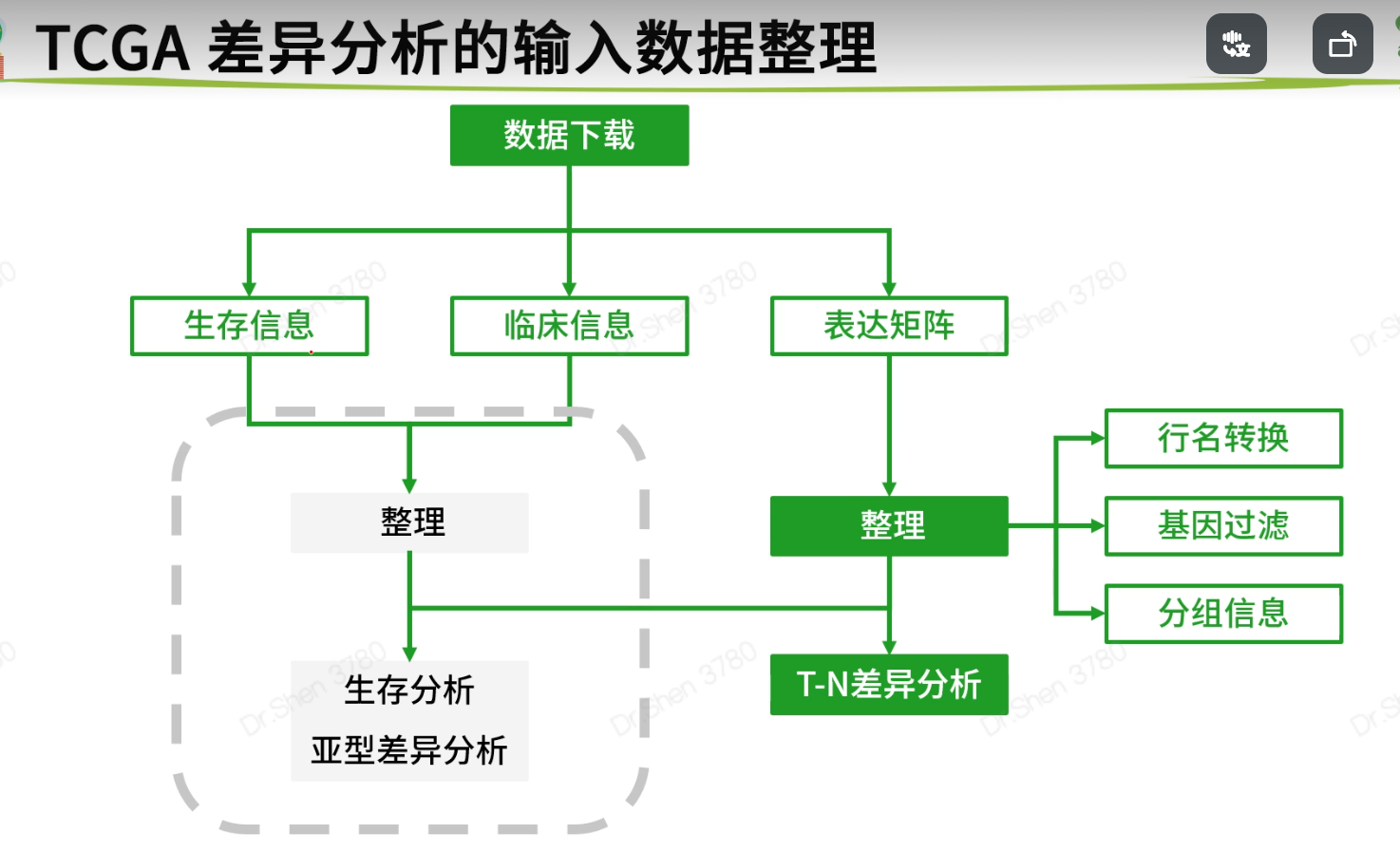
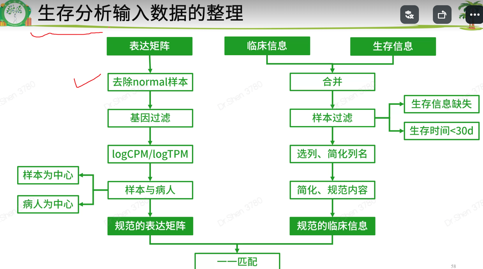
生存分析前的数据整理
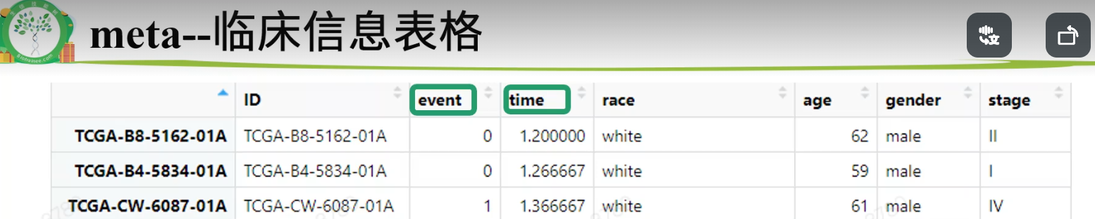
表达矩阵只需要tumor数据,不要normal,将其去掉,新表达矩阵数据命名为exprSet;临床信息需要进一步整理,成为生存分析需要的格式,新临床信息数据命名为meta。rm(list=ls())proj = "TCGA-KIRC"load(paste0(proj,".Rdata"))library(stringr)1.整理表达矩阵1.1去除normal样本table(Group)#> Group#> normal tumor#> 72 535exprSet = exp[,Group=='tumor']ncol(exp)#> [1] 607ncol(exprSet)#> [1] 5351.2 基因过滤再次进行基因过滤.(1)标准1:至少要在50%的样本里表达量大于0(最低标准)。exp(600样本)满足“至少在300个样本里表达量>0”,不能等同于 exprSet(500样本)满足“至少在250个样本里表达量>0”k = apply(exprSet,1, function(x){sum(x>0)>0.5*ncol(exprSet)});table(k)#> k#> FALSE TRUE#> 155 31798exprSet = exprSet[k,]nrow(exprSet)#> [1] 31798(2)标准2:至少在一半以上样本里表达量>10(其他数字也可,酌情调整)k = apply(exprSet,1, function(x){sum(x>10)>0.5*ncol(exprSet)});table(k)#> k#> FALSE TRUE#> 11718 20080exprSet = exprSet[k,]nrow(exprSet)#> [1] 200801.3 使用logCPM或logTPM数据exprSet[1:4,1:4]#> TCGA-BP-4342-01A TCGA-A3-3387-01A TCGA-BP-4167-01A TCGA-B8-4620-01A#> WASH7P 77 69 23 29#> AL627309.6 282 36 26 88#> WASH9P 222 147 74 47#> AP006222.1 77 23 23 14exprSet=log2(edgeR::cpm(exprSet)+1)exprSet[1:4,1:4]#> TCGA-BP-4342-01A TCGA-A3-3387-01A TCGA-BP-4167-01A TCGA-B8-4620-01A#> WASH7P 1.049412 1.0031558 0.5304210 0.5510009#> AL627309.6 2.297940 0.6078858 0.5871819 1.2698370#> WASH9P 2.029993 1.6506568 1.2807483 0.8104724#> AP006222.1 1.049412 0.4166163 0.5304210 0.29223031.4 样本与病人有的病人会有两个或两个以上的肿瘤样本,就有重复。两种可行的办法:(1)以病人为中心,对表达矩阵的列按照病人ID去重复,每个病人只保留一个样本。exprSet = exprSet[,sort(colnames(exprSet))]k = !duplicated(str_sub(colnames(exprSet),1,12));table(k)#> k#> FALSE TRUE#> 5 530exprSet = exprSet[,k]ncol(exprSet)#> [1] 530(2)以样本为中心,如果每个病人有多个样本则全部保留。(删掉上面这一段代码即可)2.整理生存信息和临床信息2.1数据合并xena单独整理了生存信息,和临床信息是分开存放的。后续构建模型可能会需要纳入一些临床信息,所以要合并到一起。library(dplyr)nrow(surv)#> [1] 979nrow(clinical)#> [1] 985meta = left_join(surv,clinical,by = c("sample"= "submitter_id.samples"))nrow(surv)#> [1] 9792.2 样本过滤去掉生存信息不全或者生存时间小于30天的样本,样本纳排标准不唯一,且差别很大k1 = meta$OS.time >= 30;table(k1)#> k1#> FALSE TRUE#> 20 959k2 = !(is.na(meta$OS.time)|is.na(meta$OS));table(k2)#> k2#> TRUE#> 979meta = meta[k1&k2,]2.3 选列、简化列名小技巧:搜索列名tmp = data.frame(colnames(meta))#View(tmp)选择需要的列,简化列名meta = meta[,c('sample','OS','OS.time','race.demographic','age_at_initial_pathologic_diagnosis','gender.demographic' ,'tumor_stage.diagnoses')]colnames(meta)=c('ID','event','time','race','age','gender','stage')str(meta)#> 'data.frame': 959 obs. of 7 variables:#> $ ID : chr "TCGA-B8-5162-01A" "TCGA-B4-5834-01A" "TCGA-CW-6087-01A" "TCGA-CW-6087-11A" ...#> $ event : int 0 0 1 1 1 1 1 1 0 1 ...#> $ time : int 36 38 41 41 42 42 43 43 43 51 ...#> $ race : chr "white" "white" "white" "white" ...#> $ age : int 62 59 61 61 75 75 65 65 35 72 ...#> $ gender: chr "male" "male" "male" "male" ...#> $ stage : chr "stage ii" "stage i" "stage iv" "stage iv" ...2.4 简化、规范内容结局事件生存分析的输入数据里,要求结局事件必须用0和1表示,1表示阳性结局。xena的数据是整理好的,其他来源的需要自行检查和整理。table(meta$event)#>#> 0 1#> 622 337#自行整理的例子:a = c("Dead", "Dead", "Alive", "Dead", "Alive")ifelse(a=="Alive",0,1)#> [1] 1 1 0 1 0生存时间认清生存时间的单位(通常是月,也可以用天和年);range(meta$time)#> [1] 36 4537meta$time = meta$time/30range(meta$time)#> [1] 1.2000 151.2333(3)检查各列的信息是否规范,没有冗余信息。缺失的信息用NA代替table(meta$stage)#>#> not reported stage i stage ii stage iii stage iv#> 4 467 101 226 161meta$stage = meta$stage %>%str_replace("not reported",as.character(NA)) %>%str_remove("stage ") %>%str_to_upper()table(meta$stage,useNA = "always")#>#> I II III IV <NA>#> 467 101 226 161 4table(meta$race)#>#> asian black or african american not reported#> 16 69 14#> white#> 860meta$race = meta$race %>%str_replace("not reported",as.character(NA))table(meta$race,useNA = "always")#>#> asian black or african american white#> 16 69 860#> <NA>#> 14table(meta$gender,useNA = "always")#>#> female male <NA>#> 327 632 0str(meta)#> 'data.frame': 959 obs. of 7 variables:#> $ ID : chr "TCGA-B8-5162-01A" "TCGA-B4-5834-01A" "TCGA-CW-6087-01A" "TCGA-CW-6087-11A" ...#> $ event : int 0 0 1 1 1 1 1 1 0 1 ...#> $ time : num 1.2 1.27 1.37 1.37 1.4 ...#> $ race : chr "white" "white" "white" "white" ...#> $ age : int 62 59 61 61 75 75 65 65 35 72 ...#> $ gender: chr "male" "male" "male" "male" ...#> $ stage : chr "II" "I" "IV" "IV" ...3.实现表达矩阵与临床信息的匹配即:meta的每一行与exprSet每一列一一对应rownames(meta) <- meta$IDs = intersect(rownames(meta),colnames(exprSet));length(s)#> [1] 513exprSet = exprSet[,s]meta = meta[s,]dim(exprSet)#> [1] 20080 513dim(meta)#> [1] 513 7identical(rownames(meta),colnames(exprSet))#> [1] TRUEsave(meta,exprSet,proj,file = paste0(proj,"_sur_model.Rdata")) #将_sur_model.Rdata弄好
实操
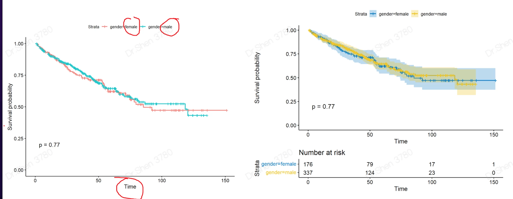
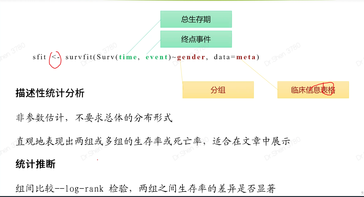
1.准备输入数据rm(list = ls())proj = "TCGA-KIRC"load(paste0(proj,"_sur_model.Rdata"))ls()#> [1] "exprSet" "meta" "proj"exprSet[1:4,1:4]#> TCGA-B8-5162-01A TCGA-B4-5834-01A TCGA-CW-6087-01A TCGA-B0-4698-01A#> WASH7P 0.38330266 1.0823971 0.24141414 0.8200756#> AL627309.6 0.04121953 0.1330091 0.60612548 1.7747381#> WASH9P 0.95751073 1.8118992 0.66255436 1.7390920#> AP006222.1 0.15825052 0.2713707 0.08503973 0.5589702str(meta)#> 'data.frame': 513 obs. of 7 variables:#> $ ID : chr "TCGA-B8-5162-01A" "TCGA-B4-5834-01A" "TCGA-CW-6087-01A" "TCGA-B0-4698-01A" ...#> $ event : int 0 0 1 1 1 0 1 0 1 0 ...#> $ time : num 1.2 1.27 1.37 1.4 1.43 ...#> $ race : chr "white" "white" "white" "white" ...#> $ age : int 62 59 61 75 65 35 72 50 84 76 ...#> $ gender: chr "male" "male" "male" "male" ...#> $ stage : chr "II" "I" "IV" "IV" ...2.KM-plot简单版本和进阶版本library(survival)library(survminer)sfit <- survfit(Surv(time, event)~gender, data=meta)ggsurvplot(sfit,pval=TRUE)ggsurvplot(sfit,palette = "jco",risk.table =TRUE,pval =TRUE,conf.int =TRUE)连续型信息怎么作KM分析?例如年龄,基因?连续型数据的离散化年龄group = ifelse(meta$age>median(meta$age,na.rm = T),"older","younger")table(group)#> group#> older younger#> 251 262sfit=survfit(Surv(time, event)~group, data=meta)ggsurvplot(sfit,pval =TRUE, data = meta, risk.table = TRUE)基因g = rownames(exprSet)[1];g#> [1] "WASH7P"meta$gene = ifelse(exprSet[g,]> median(exprSet[g,]),'high','low')sfit=survfit(Surv(time, event)~gene, data=meta)ggsurvplot(sfit,pval =TRUE, data = meta, risk.table = TRUE)

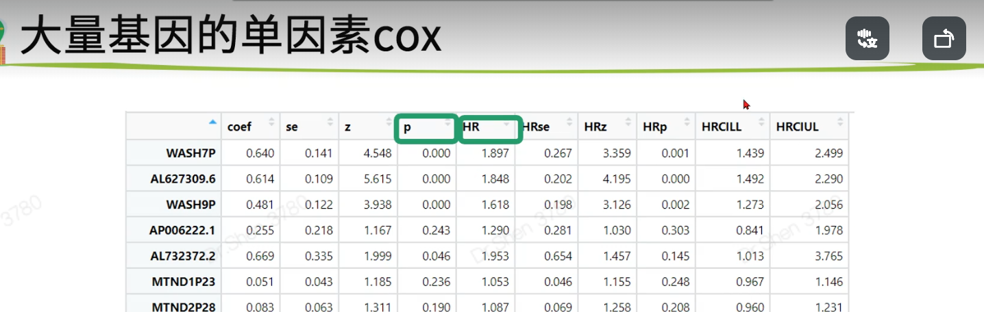
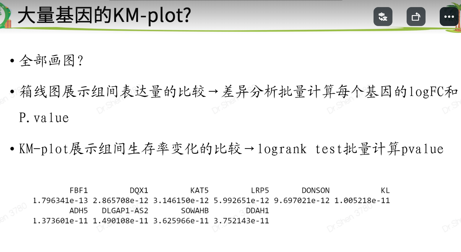
2.log-rank testKM的p值是log-rank test得出的,可批量操作source("KM_cox_function.R")logrankfile = paste0(proj,"_log_rank_p.Rdata")if(!file.exists(logrankfile)){log_rank_p <- apply(exprSet , 1 , geneKM)log_rank_p=sort(log_rank_p)save(log_rank_p,file = logrankfile)}load(logrankfile)table(log_rank_p<0.01)#>#> FALSE TRUE#> 13023 7057table(log_rank_p<0.05)#>#> FALSE TRUE#> 10232 98483.批量单因素coxcoxfile = paste0(proj,"_cox.Rdata")if(!file.exists(coxfile)){cox_results <-apply(exprSet , 1 , genecox)cox_results=as.data.frame(t(cox_results))save(cox_results,file = coxfile)}load(coxfile)table(cox_results$p<0.01)#>#> FALSE TRUE#> 11911 8169table(cox_results$p<0.05)#>#> FALSE TRUE#> 9373 10707lr = names(log_rank_p)[log_rank_p<0.01];length(lr)#> [1] 7057cox = rownames(cox_results)[cox_results$p<0.01];length(cox)#> [1] 8169length(intersect(lr,cox))#> [1] 6165save(lr,cox,file = paste0(proj,"_logrank_cox_gene.Rdata"))
KM-cox
geneKM = function(gene){meta$group=ifelse(gene>median(gene),'high','low')data.survdiff=survdiff(Surv(time, event)~group,data=meta)p.val = 1 - pchisq(data.survdiff$chisq, length(data.survdiff$n) - 1)return(p.val)}genecox = function(gene){meta$gene = gene#可直接使用连续型变量m = coxph(Surv(time, event) ~ gene, data = meta)#也可使用二分类变量#meta$group=ifelse(gene>median(gene),'high','low')#meta$group = factor(meta$group,levels = c("low","high"))#m=coxph(Surv(time, event) ~ group, data = meta)beta <- coef(m)se <- sqrt(diag(vcov(m)))HR <- exp(beta)HRse <- HR * se#summary(m)tmp <- round(cbind(coef = beta,se = se, z = beta/se,p = 1 - pchisq((beta/se)^2, 1),HR = HR, HRse = HRse,HRz = (HR - 1) / HRse,HRp = 1 - pchisq(((HR - 1)/HRse)^2, 1),HRCILL = exp(beta - qnorm(.975, 0, 1) * se),HRCIUL = exp(beta + qnorm(.975, 0, 1) * se)), 3)return(tmp['gene',])#return(tmp['grouphigh',])#二分类变量}
生存模型
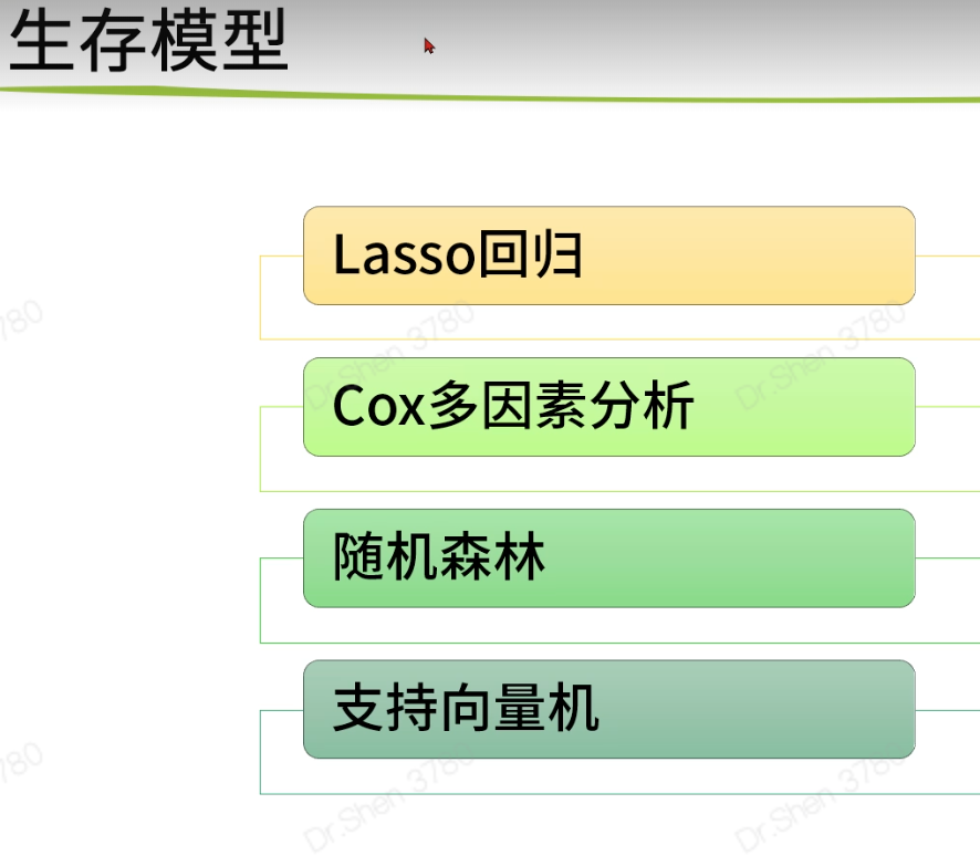
Lasso回归
作用:①将重要的基因筛选出来,
②可得出公式,得出参与基因的系数,代入后可得出风险值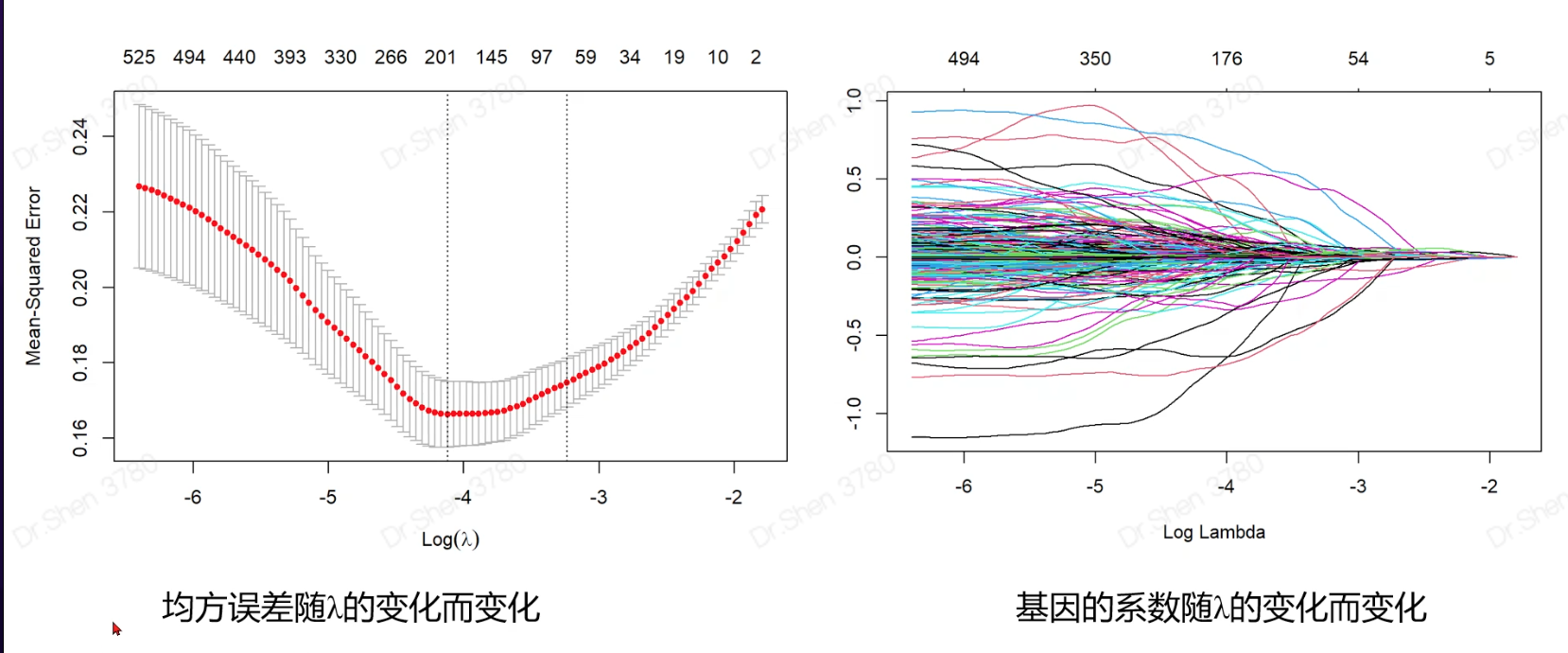
训练集和测试集不同
1.准备输入数据rm(list = ls())proj = "TCGA-KIRC"load(paste0(proj,"_sur_model.Rdata"))ls()#> [1] "exprSet" "meta" "proj"exprSet[1:4,1:4]#> TCGA-B8-5162-01A TCGA-B4-5834-01A TCGA-CW-6087-01A TCGA-B0-4698-01A#> WASH7P 0.38330266 1.0823971 0.24141414 0.8200756#> AL627309.6 0.04121953 0.1330091 0.60612548 1.7747381#> WASH9P 0.95751073 1.8118992 0.66255436 1.7390920#> AP006222.1 0.15825052 0.2713707 0.08503973 0.5589702str(meta)#> 'data.frame': 513 obs. of 7 variables:#> $ ID : chr "TCGA-B8-5162-01A" "TCGA-B4-5834-01A" "TCGA-CW-6087-01A" "TCGA-B0-4698-01A" ...#> $ event : int 0 0 1 1 1 0 1 0 1 0 ...#> $ time : num 1.2 1.27 1.37 1.4 1.43 ...#> $ race : chr "white" "white" "white" "white" ...#> $ age : int 62 59 61 75 65 35 72 50 84 76 ...#> $ gender: chr "male" "male" "male" "male" ...#> $ stage : chr "II" "I" "IV" "IV" ...load(paste0(proj,"_logrank_cox_gene.Rdata"))g = cox[1:1000] #这里是示例,取了1000个单因素cox筛选的基因,活学活用exprSet = exprSet[g,]2.构建lasso回归模型输入数据是表达矩阵(仅含tumor样本)和每个病人对应的生死(顺序必须一致)。x=t(exprSet)y=meta$eventlibrary(glmnet)#> Warning: package 'glmnet' was built under R version 4.1.3#> Warning: package 'Matrix' was built under R version 4.1.32.1挑选合适的λ值Lambda 是构建模型的重要参数。他的大小关系着模型选择的基因个数#调优参数set.seed(1006)cv_fit <- cv.glmnet(x=x, y=y)plot(cv_fit)#系数图fit <- glmnet(x=x, y=y)plot(fit,xvar = "lambda")两条虚线分别指示了两个特殊的λ值,一个是lambda.min,一个是lambda.1se,这两个值之间的lambda都认为是合适的。lambda.1se构建的模型最简单,即使用的基因数量少,而lambda.min则准确率更高一点,使用的基因数量更多一点。2.2 用这两个λ值重新建模model_lasso_min <- glmnet(x=x, y=y,lambda=cv_fit$lambda.min)model_lasso_1se <- glmnet(x=x, y=y,lambda=cv_fit$lambda.1se)选中的基因与系数存放于模型的子集beta中,用到的基因有一个s0值,没用的基因只记录了“.”,所以可以用下面代码挑出用到的基因。head(model_lasso_min$beta,20)choose_gene_min=rownames(model_lasso_min$beta)[as.numeric(model_lasso_min$beta)!=0]choose_gene_1se=rownames(model_lasso_1se$beta)[as.numeric(model_lasso_1se$beta)!=0]length(choose_gene_min)#> [1] 41length(choose_gene_1se)#> [1] 33save(choose_gene_min,file = paste0(proj,"_lasso_choose_gene_min.Rdata"))save(choose_gene_1se,file = paste0(proj,"_lasso_choose_gene_1se.Rdata"))3.模型预测和评估newx参数是预测对象。输出结果lasso.prob是一个矩阵,第一列是min的预测结果,第二列是1se的预测结果,预测结果是概率,或者说百分比,不是绝对的0和1。将每个样本的生死和预测结果放在一起,直接cbind即可。lasso.prob <- predict(cv_fit, newx=x , s=c(cv_fit$lambda.min,cv_fit$lambda.1se) )head(lasso.prob)#> s1 s2#> TCGA-B8-5162-01A 0.35441206 0.37673630#> TCGA-B4-5834-01A 0.06975962 0.07579627#> TCGA-CW-6087-01A 0.72387660 0.64176153#> TCGA-B0-4698-01A 0.63402199 0.54280316#> TCGA-B0-4690-01A 0.83592571 0.75407756#> TCGA-AS-3778-01A -0.13649093 -0.02911398ROC曲线library(pROC)library(ggplot2)m <- roc(meta$event,lasso.prob[,1])g <- ggroc(m,legacy.axes = T,size = 1,color = "#2fa1dd")auc(m)#> Area under the curve: 0.8687g + theme_bw() +geom_segment(aes(x = 0, xend = 1, y = 0, yend = 1),colour = "grey", linetype = "dashed")+annotate("text",x = .75, y = .25,label = paste("AUC of min = ",format(round(as.numeric(auc(m)),2),nsmall = 2)),color = "#2fa1dd")计算AUC取值范围在0.5-1之间,越接近于1越好。可以根据预测结果绘制ROC曲线。两个模型的曲线画在一起m2 <- roc(meta$event, lasso.prob[,2])auc(m2)#> Area under the curve: 0.8507g <- ggroc(list(min = m,se = m2),legacy.axes = T,size = 1)g + theme_bw() +scale_color_manual(values = c("#2fa1dd", "#f87669"))+geom_segment(aes(x = 0, xend = 1, y = 0, yend = 1),colour = "grey", linetype = "dashed")+annotate("text",x = .75, y = .25,label = paste("AUC of min = ",format(round(as.numeric(auc(m)),2),nsmall = 2)),color = "#2fa1dd")+annotate("text",x = .75, y = .15,label = paste("AUC of 1se = ",format(round(as.numeric(auc(m2)),2),nsmall = 2)),color = "#f87669")5.切割数据构建模型并预测5.1 切割数据(数据>500)用R包caret切割数据,生成的结果是一组代表列数的数字,用这些数字来给表达矩阵和meta取子集即可。library(caret)#> Warning: package 'caret' was built under R version 4.1.3set.seed(12345679)sam<- createDataPartition(meta$event, p = .5,list = FALSE)head(sam)#> Resample1#> [1,] 5#> [2,] 9#> [3,] 13#> [4,] 17#> [5,] 19#> [6,] 21可查看两组一些临床参数切割比例train <- exprSet[,sam]test <- exprSet[,-sam]train_meta <- meta[sam,]test_meta <- meta[-sam,]prop.table(table(train_meta$stage))#>#> I II III IV#> 0.5058824 0.1019608 0.2117647 0.1803922prop.table(table(test_meta$stage))#>#> I II III IV#> 0.4941176 0.1176471 0.2470588 0.1411765prop.table(table(test_meta$race))#>#> asian black or african american white#> 0.01587302 0.09920635 0.88492063prop.table(table(train_meta$race))#>#> asian black or african american white#> 0.01574803 0.10236220 0.881889765.2 切割后的train数据集建模和上面的建模方法一样。#计算lambdax = t(train)y = train_meta$eventcv_fit <- cv.glmnet(x=x, y=y)plot(cv_fit)#构建模型model_lasso_min <- glmnet(x=x, y=y,lambda=cv_fit$lambda.min)model_lasso_1se <- glmnet(x=x, y=y,lambda=cv_fit$lambda.1se)#挑出基因head(model_lasso_min$beta)#> 6 x 1 sparse Matrix of class "dgCMatrix"#> s0#> WASH7P .#> AL627309.6 .#> WASH9P .#> MTATP6P1 .#> LINC01409 .#> LINC00115 .choose_gene_min=rownames(model_lasso_min$beta)[as.numeric(model_lasso_min$beta)!=0]choose_gene_1se=rownames(model_lasso_1se$beta)[as.numeric(model_lasso_1se$beta)!=0]length(choose_gene_min)#> [1] 31length(choose_gene_1se)#> [1] 214.模型预测用训练集构建模型,预测测试集的生死,注意newx参数变了。lasso.prob <- predict(cv_fit, newx=t(test), s=c(cv_fit$lambda.min,cv_fit$lambda.1se) )head(lasso.prob)#> s1 s2#> TCGA-B8-5162-01A 0.39653904 0.43398261#> TCGA-B4-5834-01A 0.10082314 0.16288716#> TCGA-CW-6087-01A 0.69858720 0.63793147#> TCGA-B0-4698-01A 0.52026571 0.54582571#> TCGA-AS-3778-01A -0.02908933 0.07121892#> TCGA-B2-4098-01A 0.38169229 0.35982935再画ROC曲线library(pROC)library(ggplot2)m <- roc(test_meta$event, lasso.prob[,1])g <- ggroc(m,legacy.axes = T,size = 1,color = "#2fa1dd")auc(m)#> Area under the curve: 0.7696g + theme_bw() +geom_segment(aes(x = 0, xend = 1, y = 0, yend = 1),colour = "grey", linetype = "dashed")+annotate("text",x = .75, y = .25,label = paste("AUC of min = ",format(round(as.numeric(auc(m)),2),nsmall = 2)),color = "#2fa1dd")计算AUC取值范围在0.5-1之间,越接近于1越好。可以根据预测结果绘制ROC曲线。两个模型的曲线画在一起m2 <- roc(test_meta$event, lasso.prob[,2])auc(m2)#> Area under the curve: 0.7569g <- ggroc(list(min = m,se = m2),legacy.axes = T,size = 1)g + theme_bw() +scale_color_manual(values = c("#2fa1dd", "#f87669"))+geom_segment(aes(x = 0, xend = 1, y = 0, yend = 1),colour = "grey", linetype = "dashed")+annotate("text",x = .75, y = .25,label = paste("AUC of min = ",format(round(as.numeric(auc(m)),2),nsmall = 2)),color = "#2fa1dd")+annotate("text",x = .75, y = .15,label = paste("AUC of 1se = ",format(round(as.numeric(auc(m2)),2),nsmall = 2)),color = "#f87669")
用自己的数据进行逻辑回归- lasso分析
导入数据格式
rm(list = ls())library(glmnet)library(readxl)library(plyr)library(caret)library(corrplot)library(ggplot2)library(Hmisc)library(openxlsx)data <- read.xlsx("/Users/mac/Desktop/r/data1.xlsx")x <- as.matrix(data[,-c(1:2)])y <- as.double(data$Group)fit <- glmnet(x,y,family = "binomial",nlambda = 1000,alpha = 1)print(fit)plot(fit,xvar = "lambda")#筛选最合适的变量lasso_fit <- cv.glmnet(x,y,family="binomial",alpha = 1,type.measure = "auc",nlambda = 1000)plot(lasso_fit)print(lasso_fit)#使用lambda.lse 获取的模型较好lasso_best <- glmnet(x=x,y=y,alpha = 1,lambda = lasso_fit$lambda.1se)coef(lasso_best)coefficient <- coef(lasso_best,s=lasso_best$lambda.lse)coe <- coefficient@xcoe <- as.data.frame(coe)Active_Index <- which(as.numeric(coefficient)!=0)active_coefficients <- as.numeric(coefficient)[Active_Index]variable <- rownames(coefficient)[Active_Index]variable <- as.data.frame(variable)variable <-cbind(variable,coe)#使用lambda.min 适用于样本质量较差,纳入模型中的变量较多lasso_best <- glmnet(x=x,y=y,alpha = 1,lambda = lasso_fit$lambda.min)coef(lasso_best)coefficient <- coef(lasso_best,s=lasso_best$lambda.min)coe <- coefficient@xcoe <- as.data.frame(coe)Active_Index <- which(as.numeric(coefficient)!=0)active_coefficients <- as.numeric(coefficient)[Active_Index]variable <- rownames(coefficient)[Active_Index]variable <- as.data.frame(variable)variable <-cbind(variable,coe)
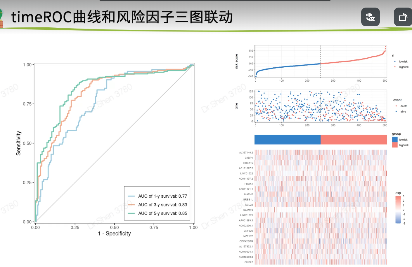
timeROC
cox-forest
1.准备输入数据rm(list = ls())proj = "TCGA-KIRC"if(!require(My.stepwise))install.packages("My.stepwise")#> Warning: package 'My.stepwise' was built under R version 4.1.3load(paste0(proj,"_sur_model.Rdata"))load(paste0(proj,"_lasso_choose_gene_1se.Rdata"))g = choose_gene_1se2.构建coxph模型将用于建模的基因(例如lasso回归选中的基因)从表达矩阵中取出来,,可作为列添加在meta表噶的后面,组成的数据框赋值给dat。library(stringr)e=t(exprSet[g,])colnames(e)= str_replace_all(colnames(e),"-","_")dat=cbind(meta,e)dat$gender=as.numeric(factor(dat$gender))dat$stage=as.numeric(factor(dat$stage))colnames(dat)#> [1] "ID" "event" "time" "race" "age"#> [6] "gender" "stage" "AL391244.2" "AJAP1" "AL357140.2"#> [11] "CPLANE2" "RCC2" "AL137127.1" "NIPAL3" "KDF1"#> [16] "LINC01389" "ANGPTL3" "GADD45A" "LINC01725" "LINC02609"#> [21] "CHI3L2" "LINC01719" "KCNN3" "MSTO1" "PMF1_BGLAP"#> [26] "CRABP2" "CD1E" "FCER1A" "NUF2" "DUTP6"#> [31] "IGFN1" "NEK2" "PROX1" "DUSP5P1" "HS1BP3_IT1"#> [36] "OTOF" "CENPA" "SLC5A6" "PRKCE" "SPTBN1"逐步回归法构建最优模型输出结果行数太多,所以我注释掉了library(survival)#> Warning: package 'survival' was built under R version 4.1.3library(survminer)# 不能允许缺失值dat2 = na.omit(dat)library(My.stepwise)vl <- colnames(dat)[c(5:ncol(dat))]# My.stepwise.coxph(Time = "time",# Status = "event",# variable.list = vl,# data = dat2)使用输出结果里的最后一个模型model = coxph(formula = Surv(time, event) ~ stage + AL357140.2 + AL391244.2 +age + OTOF + IGFN1 + CRABP2 + PMF1_BGLAP + SLC5A6 + PROX1 +LINC01719 + DUTP6, data = dat2)3.模型可视化-森林图ggforest(model,data = dat2)4.模型预测fp <- predict(model,newdata = dat2)library(Hmisc)#> Warning: package 'Hmisc' was built under R version 4.1.3options(scipen=200)with(dat2,rcorr.cens(fp,Surv(time, event))) #with函数下可将列名当作变量用#> C Index Dxy S.D. n missing#> 0.17850596(实为1- C Index 的值,故须换算) -0.64298808 0.02857663 503.00000000 0.00000000#> uncensored Relevant Pairs Concordant Uncertain#> 166.00000000 105834.00000000 18892.00000000 146654.00000000C-index用于计算生存分析中的COX模型预测值与真实之间的区分度(discrimination),也称为Harrell’s concordanceindex。C-index在0.5-1之间。0.5为完全不一致,说明该模型没有预测作用,1为完全一致,说明该模型预测结果与实际完全一致。5.切割数据构建模型并预测5.1 切割数据用R包caret切割数据,生成的结果是一组代表列数的数字,用这些数字来给表达矩阵和meta取子集即可。library(caret)#> Warning: package 'caret' was built under R version 4.1.3set.seed(12345679)sam<- createDataPartition(meta$event, p = .5,list = FALSE)train <- exprSet[,sam]test <- exprSet[,-sam]train_meta <- meta[sam,]test_meta <- meta[-sam,]5.2 切割后的train数据集建模和上面的建模方法一样。e=t(train[g,])colnames(e)= str_replace_all(colnames(e),"-","_")dat=cbind(train_meta,e)dat$gender=as.numeric(factor(dat$gender))dat$stage=as.numeric(factor(dat$stage))colnames(dat)#> [1] "ID" "event" "time" "race" "age"#> [6] "gender" "stage" "AL391244.2" "AJAP1" "AL357140.2"#> [11] "CPLANE2" "RCC2" "AL137127.1" "NIPAL3" "KDF1"#> [16] "LINC01389" "ANGPTL3" "GADD45A" "LINC01725" "LINC02609"#> [21] "CHI3L2" "LINC01719" "KCNN3" "MSTO1" "PMF1_BGLAP"#> [26] "CRABP2" "CD1E" "FCER1A" "NUF2" "DUTP6"#> [31] "IGFN1" "NEK2" "PROX1" "DUSP5P1" "HS1BP3_IT1"#> [36] "OTOF" "CENPA" "SLC5A6" "PRKCE" "SPTBN1"library(My.stepwise)dat2 = na.omit(dat)vl <- colnames(dat2)[c(5:ncol(dat2))]# My.stepwise.coxph(Time = "time",# Status = "event",# variable.list = vl,# data = dat2)model = coxph(formula = Surv(time, event) ~ stage + AL357140.2 + IGFN1 +AJAP1 + ANGPTL3 + SLC5A6 + HS1BP3_IT1 + AL137127.1 + LINC01719 +CRABP2, data = dat2)5.3 模型可视化ggforest(model, data =dat2)5.4 用切割后的数据test数据集验证模型e=t(test[g,])colnames(e)= str_replace_all(colnames(e),"-","_")test_dat=cbind(test_meta,e)test_dat$gender=as.numeric(factor(test_dat$gender))test_dat$stage=as.numeric(factor(test_dat$stage))fp <- predict(model,newdata = test_dat)library(Hmisc)with(test_dat,rcorr.cens(fp,Surv(time, event)))#> C Index Dxy S.D. n missing#> 0.22187105 -0.55625790 0.04736798 255.00000000 1.00000000#> uncensored Relevant Pairs Concordant Uncertain#> 86.00000000 28476.00000000 6318.00000000 36294.00000000

若有收获,就点个赞吧
0 人点赞
