1. Python Script algorithm

STEP1:

The first script can:

1.K-mer count:

Identify all FASTA files under the current folder, take out every K base, count each K base combination, and calculate the percentage.

Output Base Times Percent three-column matrix in CSV format.

2. Merge different samples:

Further, identify all CSV files generated in 1, and take out the Base and Percent columns.

Merge according to Base and change the column name to sample name and merge into a CSV file with base as the row name and percent as the column name.

3. Usage:

Switch cd to the directory where all fasta files are stored; Execute python kmer.py K
Enter the K value to get a mergeall.csv file. For further analysis in STPE2 R.

import argparse
def kmer(k):
    import os
    from collections import Counter
    import pandas as pd
    import globs
    FileList=os.listdir()
    for File in FileList:
        if os.path.splitext(File)[1]=='.fasta':
            f = open(File, 'r')
            lines = f.readlines()
            seq = ''
            for i in lines:
                if i[0] == '>':
                    continue
                else:
                    seq += i.strip()
            Dnuclic = (seq[start:start+k] for start in range(0, len(seq)-k+1))
            counts = Counter(Dnuclic)
            counts = dict(counts)
            counts = list(counts.items())
            data = pd.DataFrame(counts, columns=['Base', 'Times'])
            print(data.iloc[:, 1].sum())
            percent = data.iloc[:, 1] / (data.iloc[:, 1].sum()) * 100
            print(percent)
            data["Percent"] = percent
            data=data.drop(columns='Times')
            print(data)
            name = os.path.splitext(File)[0] + '.csv'
            data.to_csv(name, encoding='gbk')
            f.close()
    pa=os.getcwd()
    file = glob.glob(os.path.join(pa, "*.csv"))
    quanname=file[0].split("/")[-1]
    name=os.path.splitext(quanname)[0]
    df1=pd.read_csv(file[0],names=['Base',name+'Percent'],index_col=0)
    for f in file:
        qname=f.split("/")[-1]
        oname=os.path.splitext(qname)[0]
        df=pd.read_csv(f,names=['Base',name+'Percent'],index_col=0)
        df1=pd.merge(df1,df,on='Base')
    print(df1)
    df1.to_csv("mergeall.csv")
if __name__ == "__main__":
    parser = argparse.ArgumentParser()
    parser.add_argument("k", type=int, help="import your designed k value here")
    args = parser.parse_args()
    kmer(args.k)

STEP2:

Script in the second R language can carry out correlation analysis and heat map visualization for CSV containing different samples and different K combinations after combination

library(readr)
library(corrplot)
library(pheatmap)
mergeall <- read_csv("mergeall.csv")
df=as.data.frame(mergeall)
rownames(df)=df[,1]
df2=df[,-1]
M <- cor(df2)
g <- corrplot(M,method = "color")
pheatmap(M,display_numbers=T,fontsize=15) 
pheatmap(df2,show_colnames =T,show_rownames = T, cluster_cols = T,display_numbers=T,fontsize=10)
pheatmap(scale(df2),show_colnames =T,show_rownames = T, cluster_cols = T,display_numbers=T,fontsize=10)

STPE3：

Results analysis

1. Correlation of different samples:

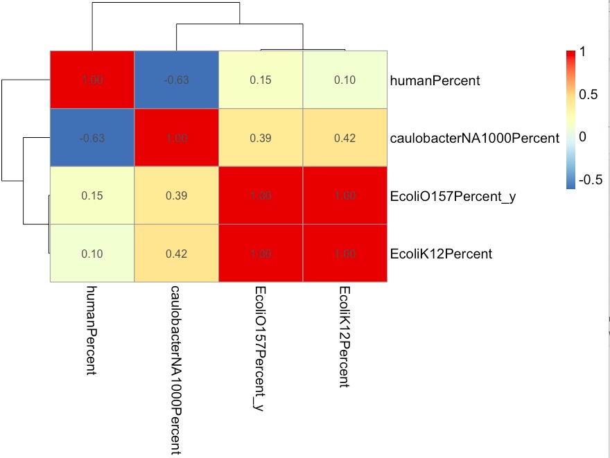
The higher the correlation, the more similar the genome was.

2. Clustering analysis of different samples K combined heat map:

We can see here:
1. In the genes of human chromosomes, The AAA and TTT sequences are significantly higher than those of other species, which is consistent with the PolyA sites in the human genome.
2. In human chromosome genes, the sequences that appear blue and are less than those of other species are base combinations with more GC: TCG, ACG, CGA, CGC, CCG, GGC, GCC.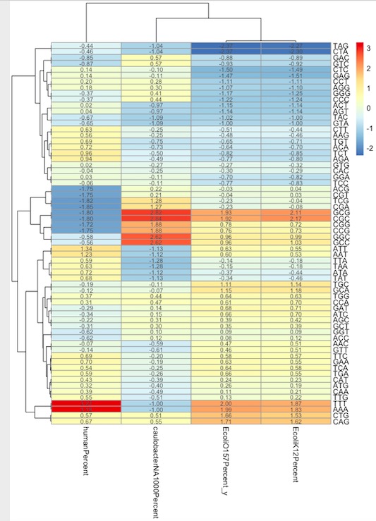

2. R language N-Gram algorithm Package:

library(ngram)
s=readLines("./Desktop/caulobacterNA1000.txt")
s2=splitter(concatenate(s,collapse =""), split.char = TRUE )
ng=ngram(s3,n=3)
M=get.phrasetable(ng)

Output matrix: